Interpolation II 8 4 SPLINE INTERPOLATION 8 5

Interpolation II (8. 4 SPLINE INTERPOLATION) (8. 5 MATLAB’s INTERPOLATION Functions) 2005. 11 2003010482 Mohiuddin Ahmad 2005010207 SUNG-BONG JANG

8. 4 : Spline Interpolation Mohiuddin Ahmad (mohi@image. korea. ac. kr) ID: 2003010482 Computer Vision and Pattern Recognition Lab. Dept. of Computer Science and Engineering Korea University Computer Vision and Pattern Recognition Lab.

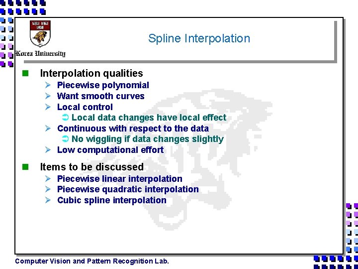
Spline Interpolation n Interpolation qualities Ø Piecewise polynomial Ø Want smooth curves Ø Local control Ü Local data changes have local effect Ø Continuous with respect to the data Ü No wiggling if data changes slightly Ø Low computational effort n Items to be discussed Ø Piecewise linear interpolation Ø Piecewise quadratic interpolation Ø Cubic spline interpolation Computer Vision and Pattern Recognition Lab.

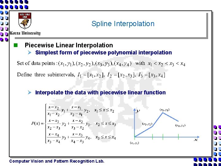
Spline Interpolation n Piecewise Linear Interpolation Ø Simplest form of piecewise polynomial interpolation Ø Interpolate the data with piecewise linear function Computer Vision and Pattern Recognition Lab.

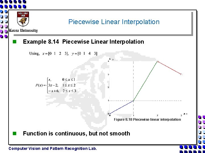
Piecewise Linear Interpolation n Example 8. 14 Piecewise Linear Interpolation Figure 8. 18 Piecewise linear interpolation n Function is continuous, but not smooth Computer Vision and Pattern Recognition Lab.

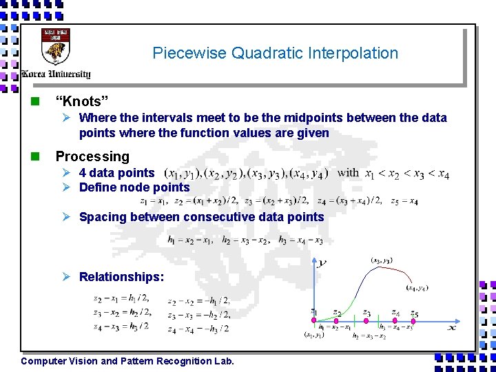
Piecewise Quadratic Interpolation n “Knots” Ø Where the intervals meet to be the midpoints between the data points where the function values are given n Processing Ø 4 data points Ø Define node points Ø Spacing between consecutive data points Ø Relationships: Computer Vision and Pattern Recognition Lab.

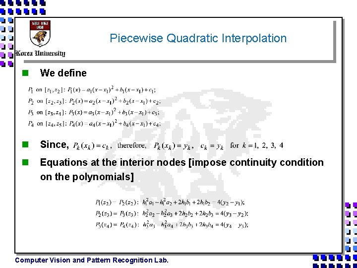
Piecewise Quadratic Interpolation n We define n Since, n Equations at the interior nodes [impose continuity condition on the polynomials] Computer Vision and Pattern Recognition Lab.

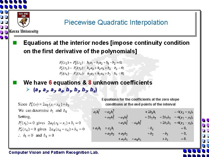
Piecewise Quadratic Interpolation n Equations at the interior nodes [impose continuity condition on the first derivative of the polynomials] n We have 6 equations & 8 unknown coefficients Ø (a 1, a 2, a 3, a 4, b 1, b 2, b 3, b 4) Equations for the coefficients at the zero slope conditions at the end points of the interval Computer Vision and Pattern Recognition Lab.

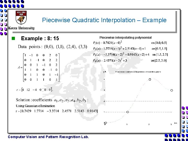
Piecewise Quadratic Interpolation – Example n Example : 8: 15 Computer Vision and Pattern Recognition Lab. Piecewise interpolating polynomial

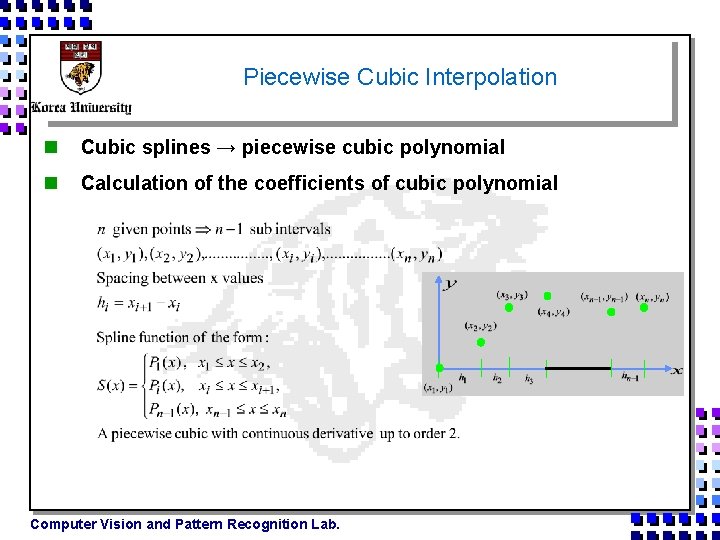
Piecewise Cubic Interpolation n Cubic splines → piecewise cubic polynomial n Calculation of the coefficients of cubic polynomial Computer Vision and Pattern Recognition Lab.

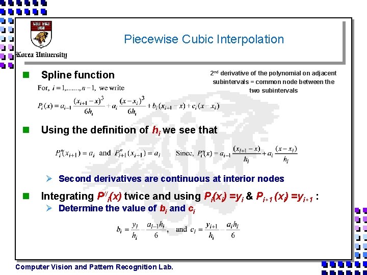
Piecewise Cubic Interpolation n Spline function n Using the definition of hi we see that 2 nd derivative of the polynomial on adjacent subintervals = common node between the two subintervals Ø Second derivatives are continuous at interior nodes n Integrating P//i(x) twice and using Pi(xi) =yi & Pi+1 (xi) =yi+1 : Ø Determine the value of bi and ci Computer Vision and Pattern Recognition Lab.

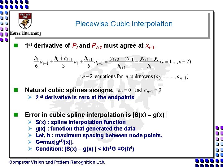
Piecewise Cubic Interpolation n 1 st derivative of Pi and Pi+1 must agree at xi+1 n Natural cubic splines assigns, Ø 2 nd derivative is zero at the endpoints n Error in cubic spline interpolation is |S(x) – g(x) | Ø Ø Ø S(x) : spline interpolation function g(x) : function that generated the data Let, h : maximum spacing between node points, G=max|g(4)(x)|. Condition: |S(x) – g(x) | < kh 4 G =O(h 4) Computer Vision and Pattern Recognition Lab.

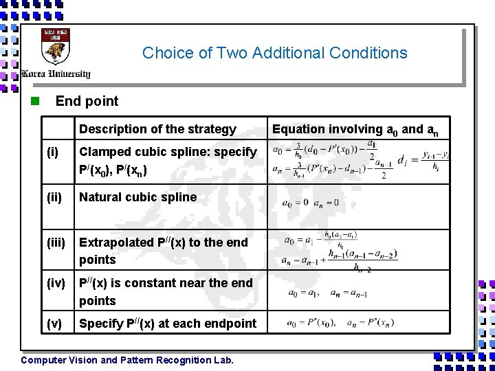
Choice of Two Additional Conditions n End point Description of the strategy (i) Clamped cubic spline: specify P/(x 0), P/(xn) (ii) Natural cubic spline (iii) Extrapolated P//(x) to the end points (iv) P//(x) is constant near the end points (v) Specify P//(x) at each endpoint Computer Vision and Pattern Recognition Lab. Equation involving a 0 and an

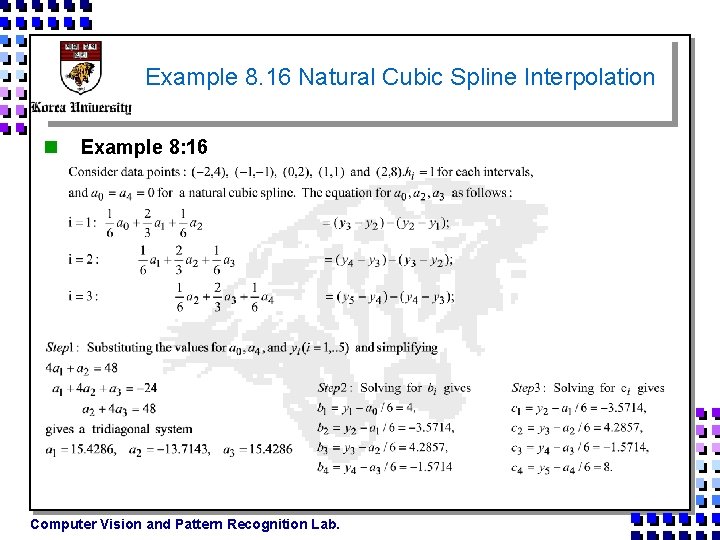
Example 8. 16 Natural Cubic Spline Interpolation n Example 8: 16 Computer Vision and Pattern Recognition Lab.

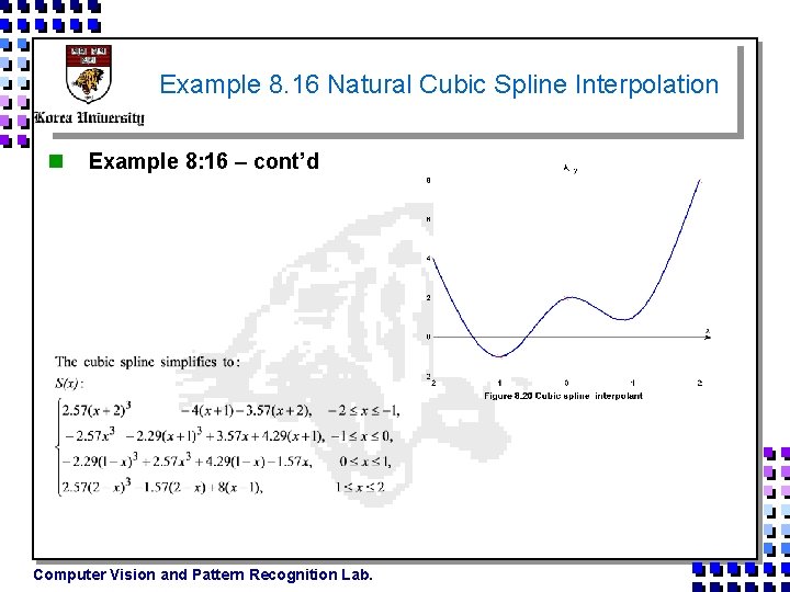
Example 8. 16 Natural Cubic Spline Interpolation n Example 8: 16 – cont’d Computer Vision and Pattern Recognition Lab.

Code for Spline Cubic Interpolation n Matlab code for i=2 : n-2 s 1=[]; s 2=[]; s 3=[]; s 4=[]; function x = tridiag(U, D, L, R) function s = spline(xx, yy) fprintf('n Resulting piecewise function: nn'); %solve Ax=b , where A os a tridiagonal matrix n = length (xx); s 1 = [sprintf('(%f)*((%f)-x). ^3/(%f)', a(i-1), xx(i+1), 6*h(i))]; %Input h(1: n-1)=xx(2: n)- xx(1: n-1); s 2 = [sprintf('(%f)*(x-(%f)). ^3/(%f)', a(i), xx(i), 6*h(i))]; % U: upper diagonal matrix A, u(n)=0 T(1: n-1)=(yy(2: n) - yy(1: n-1)). /h(1: n-1); s 3 = [sprintf('(%f)*((%f)-x)', b(i), xx(i+1))]; % D: diagonal of matrix A R(1: n-2)=T(2: n-1) - T(1: n-2); s 4 = [sprintf('(%f)*(x-(%f))', c(i), xx(i))]; % L: lower diagonal of matrix A, l(1)=0 U(1: n-3)=h(2: n-2)/6; % R: right hand side of equation D(1: n-2)=(h(1: n-2) + h(2: n-1))/3; x = xx(i): (xx(i+1)-xx(i))/10 : xx(i+1); n = length(D); L(1: n-3)=h(2: n-2)/6 ; y = eval(s 1) + eval(s 2) + eval(s 3) + eval(s 4); U(1)=U(1)/D(1); a = tridiag(U, D, L, R); xxx = [xxx x]; R(1)=R(1)/D(1); b(1)=yy(1)/h(1); yyy = [yyy y]; %U(: ); c(1)=yy(2)/h(1)- a(1)*h(1)/6; b(2: n-2)=yy(2: n-2). /h(2: n-2) - a(1: n-3). *h(2: n-2)/6; end s 1=[]; s 2=[]; s 3=[]; c(2: n-2)=yy(3: n-1). /h(2: n-2) - a(2: n-2). *h(2: n-2)/6; b(n-1)=yy(n-1)/h(n-1) - a(n-2)*h(n-1)/6; c(n-1)=yy(n)/h(n-1); U(1: n) = [U(: ) ; 0]; L(1: n) = [0 ; L(: )]; for i=2: n-1 fprintf('n Resulting piecewise function: nn'); s 1 = [sprintf('(%f)*((%f)-x). ^3/(%f)', a(n-2), xx(n), 6*h(n-1))]; denom = D(i) - L(i)*U(i-1); if(denom==0), error('zero in denominator'), end %% print piecewise function and plot it s 2 = [sprintf('(%f)*((%f)-x)', b(n-1), xx(n))]; U(i)=U(i)/denom; fprintf('n. Resulting piecewise function: nn'); s 3 = [sprintf('(%f)*(x-(%f))', c(n-1), xx(n-1))]; R(i)=(R(i)- L(i)*R(i-1))/denom; s 1 = [sprintf('(%f)*(x-(%f)). ^3/(%f)', a(1), xx(1), 6*h(1) )]; end s 2 = [sprintf('(%f)*((%f)- x)', b(1), xx(2))]; x = xx(n-1): (xx(n)-xx(n-1))/10 : xx(n); R(n)=(R(n) - L(n)*R(n-1)) / ( D(n) - L(n)*U(n-1)); s 3 = [sprintf('(%f)*(x-(%f))', c(1), xx(1))]; y = eval(s 1) + eval(s 2) + eval(s 3); x(n)=R(n); x = xx(1): (xx(2) - xx(1))/10 : xx(2); xxx = [xxx x]; for i=n-1: 1 y = eval(s 1) + eval(s 2) + eval(s 3); yyy = [yyy y]; xxx = x; plot(xxx, yyy); hold on; yyy = y; plot (xx, yy, 'r*'); hold off Computer Vision and Pattern Recognition Lab. x(i)= R(i) - U(i)*x(i+1); end

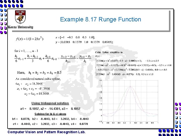
Example 8. 17 Runge Function Using tridiagonal solution a 1 = 8. 1857, a 2 = -14. 4381, a 3 = 8. 1857 Solving for bi & ci gives b 1 = 0. 0770, b 2 = -0. 4043, b 3 = c 1 = -0. 4043, c 2 = 3. 2032, b 4 = -0. 4043 3. 2032, c 3 = -0. 4043, c 4 = 0. 0770 Computer Vision and Pattern Recognition Lab.

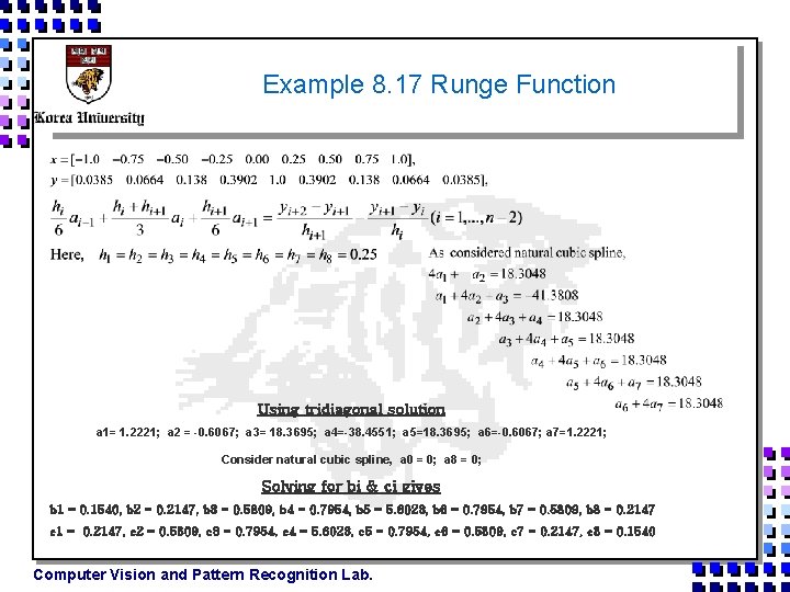
Example 8. 17 Runge Function Using tridiagonal solution a 1= 1. 2221; a 2 = -0. 6067; a 3= 18. 3695; a 4=-38. 4551; a 5=18. 3695; a 6=-0. 6067; a 7=1. 2221; Consider natural cubic spline, a 0 = 0; a 8 = 0; Solving for bi & ci gives b 1 = 0. 1540, b 2 = 0. 2147, b 3 = 0. 5809, b 4 = 0. 7954, b 5 = 5. 6023, b 6 = 0. 7954, b 7 = 0. 5809, b 8 = 0. 2147 c 1 = 0. 2147, c 2 = 0. 5809, c 3 = 0. 7954, c 4 = 5. 6023, c 5 = 0. 7954, c 6 = 0. 5809, c 7 = 0. 2147, c 8 = 0. 1540 Computer Vision and Pattern Recognition Lab.

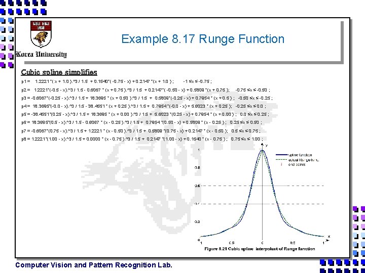
Example 8. 17 Runge Function Cubic spline simplifies p 1 = 1. 2221 *( x + 1. 0 ). ^3 / 1. 5 + 0. 1540*( -0. 75 - x) + 0. 2147 *(x + 1. 0 ) ; -1 ≤x ≤ -0. 75 ; p 2 = 1. 2221*(-0. 5 - x). ^3 / 1. 5 - 0. 6067 * (x + 0. 75 ). ^3 / 1. 5 + 0. 2147*( -0. 50 - x) + 0. 5809 *(x + 0. 75 ); -0. 75 ≤x ≤ -0. 50 ; p 3 = -0. 6067*(-0. 25 - x). ^3 / 1. 5 + 18. 3695 * (x + 0. 50 ). ^3 / 1. 5 + 0. 5809*(-0. 25 - x) + 0. 7954 * (x + 0. 5 ) ; -0. 50 ≤x ≤ -0. 25 ; p 4 = 18. 3695*(-0. 0 - x). ^3 / 1. 5 - 38. 4551 * (x + 0. 25 ). ^3 / 1. 5 + 0. 7954 *(-0. 0 - x) + 5. 6023 * (x + 0. 25 ); -0. 25 ≤x ≤ 0. 0 ; p 5 = -38. 4551*(0. 25 - x). ^3 / 1. 5 + 18. 3695 * (x + 0. 00 ). ^3 / 1. 5 + 5. 6023 *(0. 25 - x) + 0. 7954 * (x + 0. 00 ) ; 0. 0 ≤x ≤ 0. 25 ; p 6 = 18. 3695*(0. 5 - x). ^3 / 1. 5 - 0. 6067 * (x - 0. 25 ). ^3 / 1. 5 + 0. 7954 *(0. 50 - x) + 0. 5809 * (x - 0. 25 ) ; 0. 25 ≤x ≤ 0. 50 ; p 7 = -0. 6067*(0. 75 - x). ^3 / 1. 5 + 1. 2221 * (x - 0. 50 ). ^3 / 1. 5 + 0. 5809 *(0. 75 - x) + 0. 2147 * (x - 0. 50 ); 0. 5 ≤x ≤ 0. 75 ; p 8 = 1. 2221*(1. 00 - x). ^3 / 1. 5 + 0. 0000 * (x - 0. 75 ). ^3 / 1. 5 + 0. 2147 *(1. 00 - x) + 0. 1540 * (x - 0. 75 ) ; 0. 75 ≤x ≤ 1. 00 ; Computer Vision and Pattern Recognition Lab.

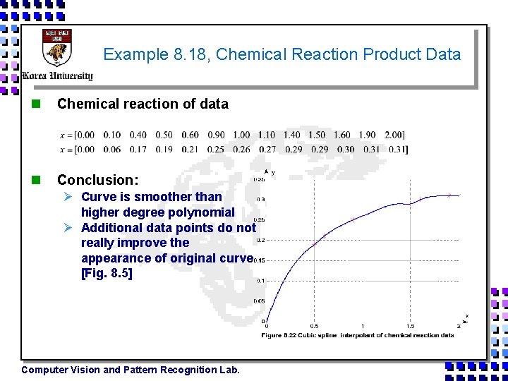
Example 8. 18, Chemical Reaction Product Data n Chemical reaction of data n Conclusion: Ø Curve is smoother than higher degree polynomial Ø Additional data points do not really improve the appearance of original curve [Fig. 8. 5] Computer Vision and Pattern Recognition Lab.

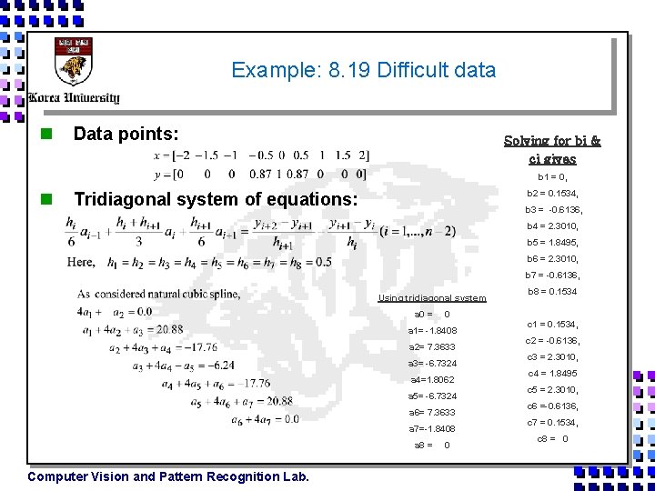
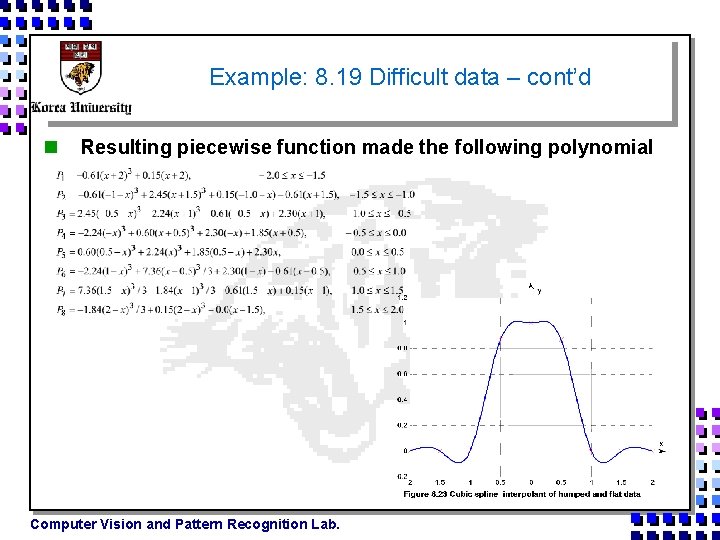
Example: 8. 19 Difficult data n Data points: Solving for bi & ci gives b 1 = 0, n b 2 = 0. 1534, Tridiagonal system of equations: b 3 = -0. 6136, b 4 = 2. 3010, b 5 = 1. 8495, b 6 = 2. 3010, b 7 = -0. 6136, Using tridiagonal system a 0 = 0 a 1= -1. 8408 a 2= 7. 3633 a 3= -6. 7324 a 4=1. 8062 a 5= -6. 7324 a 6= 7. 3633 a 7=-1. 8408 a 8 = Computer Vision and Pattern Recognition Lab. b 8 = 0. 1534 0 c 1 = 0. 1534, c 2 = -0. 6136, c 3 = 2. 3010, c 4 = 1. 8495 c 5 = 2. 3010, c 6 =-0. 6136, c 7 = 0. 1534, c 8 = 0

Example: 8. 19 Difficult data – cont’d n Resulting piecewise function made the following polynomial Computer Vision and Pattern Recognition Lab.

Interpolation II (8. 5, MATLAB’s INTERPOLATION Functions) 2005. 11 2005010207 SUNG-BONG JANG

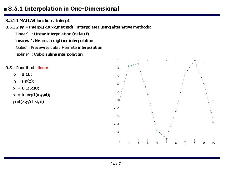
■ 8. 5. 1 Interpolation in One-Dimensional 8. 5. 1. 1 MATLAB function : Interp 1 8. 5. 1. 2 yy = interp 1(x, y, xx, method) : interpolates using alternative methods: ‘linear‘ : Linear interpolation (default) 'nearest‘ : Nearest neighbor interpolation ‘cubic’ : Piecewise cubic Hermite interpolation 'spline‘ : Cubic spline interpolation 8. 5. 1. 3 method : linear x = 0: 10; y = sin(x); xi = 0: . 25: 10; yi = interp 1(x, y, xi); plot(x, y, 'o', xi, yi) 24 / 7

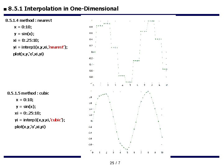
■ 8. 5. 1 Interpolation in One-Dimensional 8. 5. 1. 4 method : nearest x = 0: 10; y = sin(x); xi = 0: . 25: 10; yi = interp 1(x, y, xi, ’nearest’); plot(x, y, 'o', xi, yi) 8. 5. 1. 5 method : cubic x = 0: 10; y = sin(x); xi = 0: . 25: 10; yi = interp 1(x, y, xi, ’cubic’); plot(x, y, 'o', xi, yi) 25 / 7

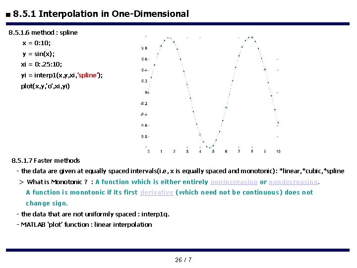
■ 8. 5. 1 Interpolation in One-Dimensional 8. 5. 1. 6 method : spline x = 0: 10; y = sin(x); xi = 0: . 25: 10; yi = interp 1(x, y, xi, ’spline’); plot(x, y, 'o', xi, yi) 8. 5. 1. 7 Faster methods - the data are given at equally spaced intervals(i. e, x is equally spaced and monotonic): *linear, *cubic, *spline > What is Monotonic ? : A function which is either entirely nonincreasing or nondecreasing. A function is monotonic if its first derivative (which need not be continuous) does not change sign. - the data that are not uniformly spaced : interp 1 q. - MATLAB ‘plot’ function : linear interpolation 26 / 7

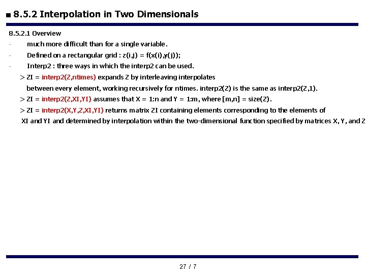
■ 8. 5. 2 Interpolation in Two Dimensionals 8. 5. 2. 1 Overview - much more difficult than for a single variable. - Defined on a rectangular grid : z(i, j) = f(x(i), y(j)); - Interp 2 : three ways in which the interp 2 can be used. > ZI = interp 2(Z, ntimes) expands Z by interleaving interpolates between every element, working recursively for ntimes. interp 2(Z) is the same as interp 2(Z, 1). > ZI = interp 2(Z, XI, YI) assumes that X = 1: n and Y = 1: m, where [m, n] = size(Z). > ZI = interp 2(X, Y, Z, XI, YI) returns matrix ZI containing elements corresponding to the elements of XI and YI and determined by interpolation within the two-dimensional function specified by matrices X, Y, and Z. 27 / 7

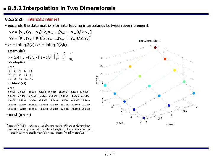
■ 8. 5. 2 Interpolation in Two Dimensionals 8. 5. 2. 2 ZI = interp 2(Z, ntimes) - expands the data matrix z by interleaving interpolanes between every element. xx = [x 1, (x 2 + x 2)/2, x 2, …. , (xn-1 + xn-1)/2, xn ] yy = [y 1, (y 2 + y 2)/2, y 2, …. , (yn-1 + yn-1)/2, yn ] - zz = interp 2(z); zz = interp 2(z, k) - Example) x=[2, 4], y =[3, 5, 7], z= x’y, >> interp 2(z) ans = 6 8 10 12 14 9 12 15 18 21 12 16 20 24 28 >> interp 2(z, 2) ans = 6. 0000 7. 0000 8. 0000 9. 0000 10. 0000 11. 0000 12. 0000 13. 0000 14. 0000 7. 5000 8. 7500 10. 0000 11. 2500 12. 5000 13. 7500 15. 0000 16. 2500 17. 5000 9. 0000 10. 5000 12. 0000 13. 5000 15. 0000 16. 5000 18. 0000 19. 5000 21. 0000 10. 5000 12. 2500 14. 0000 15. 7500 17. 5000 19. 2500 21. 0000 22. 7500 24. 5000 12. 0000 14. 0000 16. 0000 18. 0000 20. 0000 22. 0000 24. 0000 26. 0000 28. 0000 - mesh(x, y, z’) * mesh(X, Y, Z) : draws a wireframe mesh with color determined by Z so color is proportional to surface height. If X and Y are vectors, length(X) = n and length(Y) = m, where [m, n] = size(Z). 28 / 7

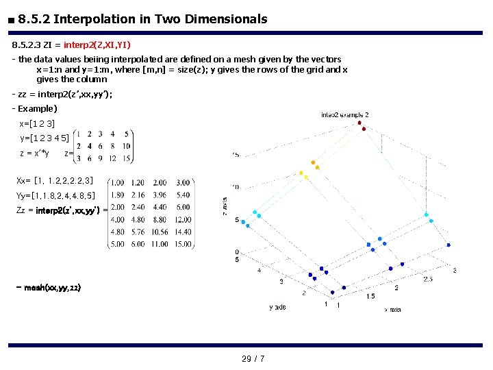
■ 8. 5. 2 Interpolation in Two Dimensionals 8. 5. 2. 3 ZI = interp 2(Z, XI, YI) - the data values beiing interpolated are defined on a mesh given by the vectors x=1: n and y=1: m, where [m, n] = size(z); y gives the rows of the grid and x gives the column - zz = interp 2(z’, xx, yy’); - Example) x=[1 2 3] y=[1 2 3 4 5] z = x’*y z= Xx= [1, 1. 2, 2, 2. 2, 3] Yy=[1, 1. 8, 2, 4, 4. 8, 5] Zz = interp 2(z’, xx, yy’) = - mesh(xx, yy, zz) 29 / 7

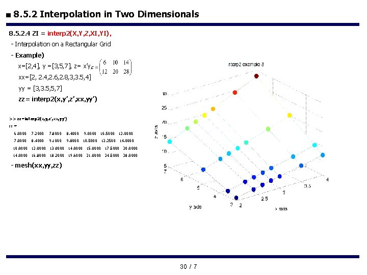
■ 8. 5. 2 Interpolation in Two Dimensionals 8. 5. 2. 4 ZI = interp 2(X, Y, Z, XI, YI), - Interpolation on a Rectangular Grid - Example) x=[2, 4], y =[3, 5, 7], z= x’y, xx=[2, 2. 4, 2. 6, 2. 8, 3, 3. 5, 4] yy = [3, 3. 5, 5, 7] zz= interp 2(x, y’, z’, xx, yy’) >> zz=interp 2(x, y, z', xx, yy') zz = 6. 0000 7. 2000 7. 8000 8. 4000 7. 0000 8. 4000 9. 1000 9. 8000 10. 5000 12. 2500 14. 0000 9. 0000 10. 5000 12. 0000 10. 0000 12. 0000 13. 0000 14. 0000 15. 0000 17. 5000 20. 0000 14. 0000 16. 8000 18. 2000 19. 6000 21. 0000 24. 5000 28. 0000 - mesh(xx, yy, zz) 30 / 7

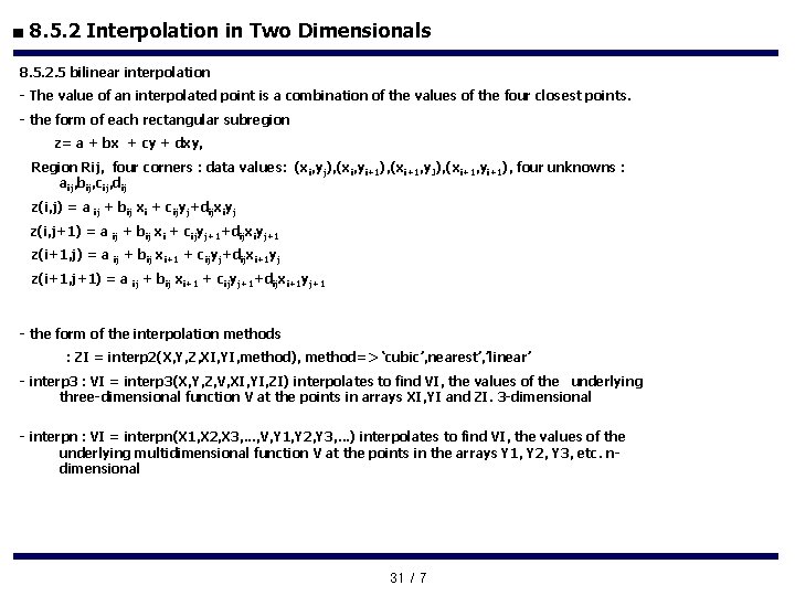
■ 8. 5. 2 Interpolation in Two Dimensionals 8. 5. 2. 5 bilinear interpolation - The value of an interpolated point is a combination of the values of the four closest points. - the form of each rectangular subregion z= a + bx + cy + dxy, Region Rij, four corners : data values: (xi, yj), (xi, yi+1), (xi+1, y. J), (xi+1, yi+1), four unknowns : aij, bij, cij, dij z(i, j) = a ij + bij xi + cijyj+dijxiyj z(i, j+1) = a ij + bij xi + cijyj+1+dijxiyj+1 z(i+1, j) = a ij + bij xi+1 + cijyj+dijxi+1 yj z(i+1, j+1) = a ij + bij xi+1 + cijyj+1+dijxi+1 yj+1 - the form of the interpolation methods : ZI = interp 2(X, Y, Z, XI, YI, method), method=> ‘cubic’, nearest’, ’linear’ - interp 3 : VI = interp 3(X, Y, Z, V, XI, YI, ZI) interpolates to find VI, the values of the underlying three-dimensional function V at the points in arrays XI, YI and ZI. 3 -dimensional - interpn : VI = interpn(X 1, X 2, X 3, . . . , V, Y 1, Y 2, Y 3, . . . ) interpolates to find VI, the values of the underlying multidimensional function V at the points in the arrays Y 1, Y 2, Y 3, etc. ndimensional 31 / 7