Internet Applications Performance Metrics and performancerelated concepts E

Internet Applications: Performance Metrics and performance-related concepts E 0397 – Lecture 2 10/8/2010

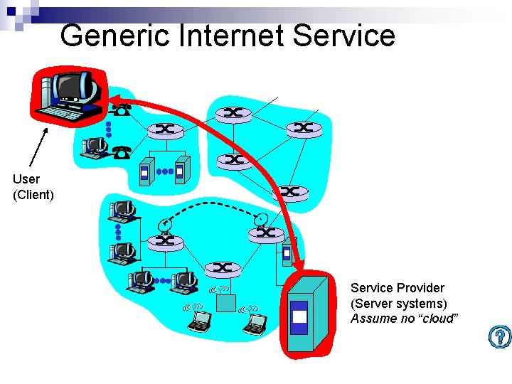
Generic Internet Service Client User (Client) Service Provider (Server systems) Assume no “cloud” Server

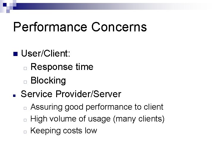
Performance Concerns n n User/Client: ¨ Response time ¨ Blocking Service Provider/Server ¨ ¨ ¨ Assuring good performance to client High volume of usage (many clients) Keeping costs low

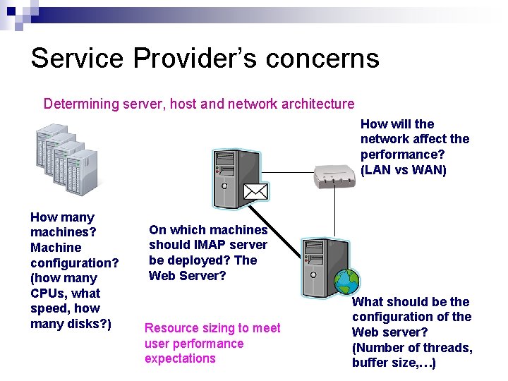
Service Provider’s concerns Determining server, host and network architecture How will the network affect the performance? (LAN vs WAN) How many machines? Machine configuration? (how many CPUs, what speed, how many disks? ) On which machines should IMAP server be deployed? The Web Server? Resource sizing to meet user performance expectations What should be the configuration of the Web server? (Number of threads, buffer size, …)

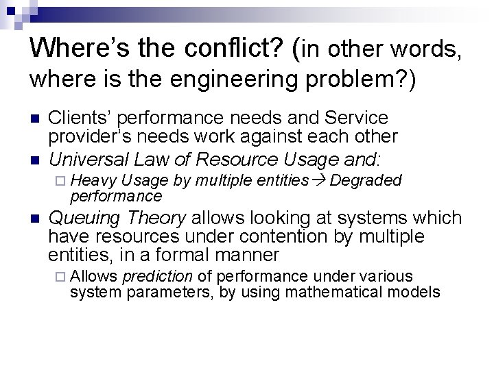
Where’s the conflict? (in other words, where is the engineering problem? ) n n Clients’ performance needs and Service provider’s needs work against each other Universal Law of Resource Usage and: Usage by multiple entities Degraded performance ¨ Heavy n Queuing Theory allows looking at systems which have resources under contention by multiple entities, in a formal manner ¨ Allows prediction of performance under various system parameters, by using mathematical models

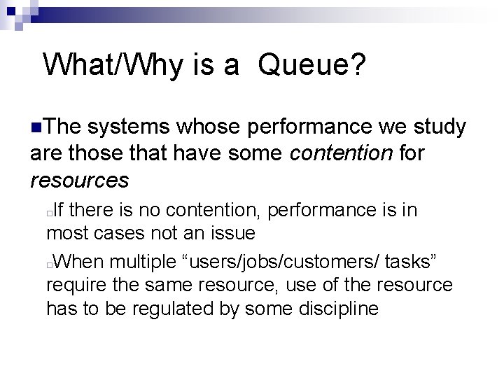
What/Why is a Queue? n. The systems whose performance we study are those that have some contention for resources If there is no contention, performance is in most cases not an issue When multiple “users/jobs/customers/ tasks” require the same resource, use of the resource has to be regulated by some discipline ¨ ¨

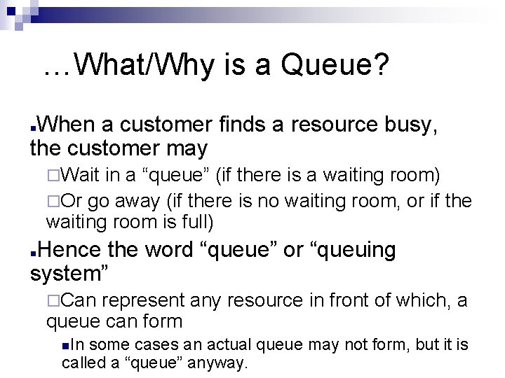
…What/Why is a Queue? When a customer finds a resource busy, the customer may n ¨Wait in a “queue” (if there is a waiting room) ¨Or go away (if there is no waiting room, or if the waiting room is full) Hence the word “queue” or “queuing system” n ¨Can represent any resource in front of which, a queue can form n. In some cases an actual queue may not form, but it is called a “queue” anyway.

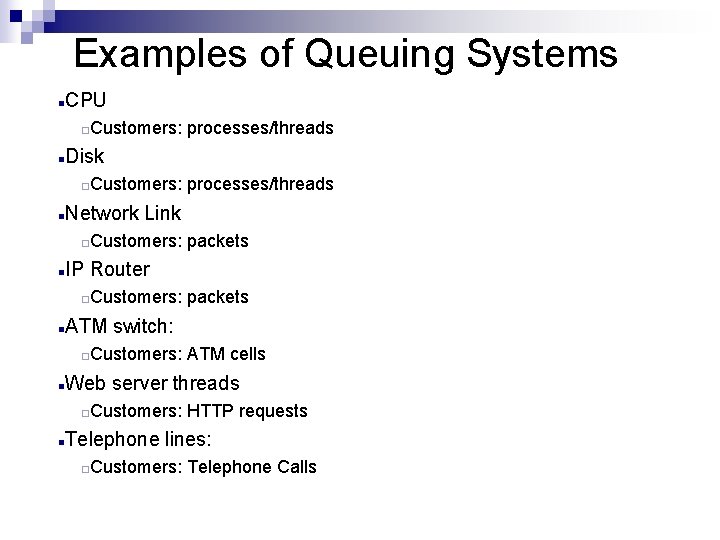
Examples of Queuing Systems CPU n Customers: processes/threads ¨ Disk n Customers: processes/threads ¨ Network Link n Customers: packets ¨ IP Router n Customers: packets ¨ ATM switch: n Customers: ATM cells ¨ Web server threads n Customers: HTTP requests ¨ Telephone lines: n Customers: Telephone Calls ¨

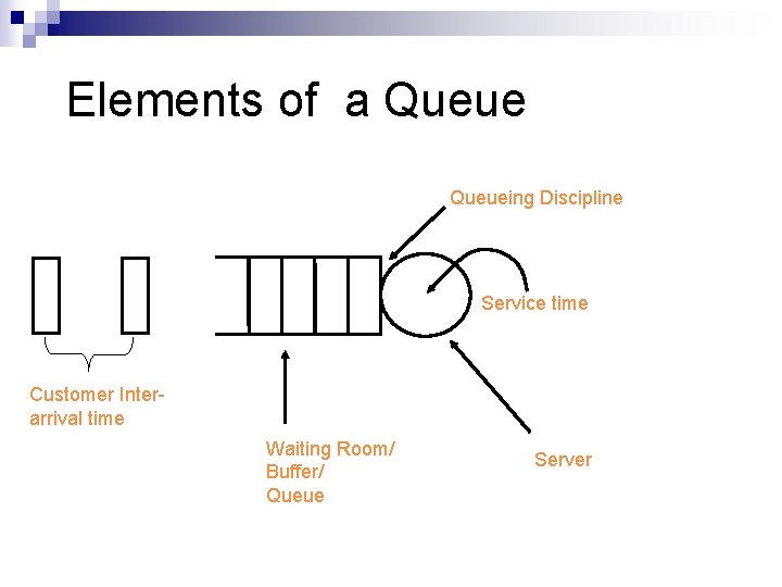
Elements of a Queueing Discipline Service time Customer Interarrival time Waiting Room/ Buffer/ Queue Server

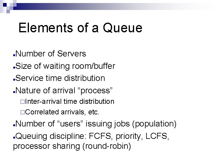
Elements of a Queue n n Number of Servers Size of waiting room/buffer Service time distribution Nature of arrival “process” ¨Inter-arrival time distribution ¨Correlated arrivals, etc. Number of “users” issuing jobs (population) Queuing discipline: FCFS, priority, LCFS, processor sharing (round-robin) n n

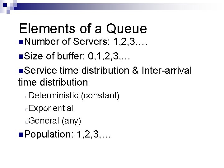
Elements of a Queue n. Number of Servers: 1, 2, 3…. n. Size of buffer: 0, 1, 2, 3, … n. Service time distribution & Inter-arrival time distribution Deterministic (constant) Exponential General (any) ¨ ¨ ¨ n. Population: 1, 2, 3, …

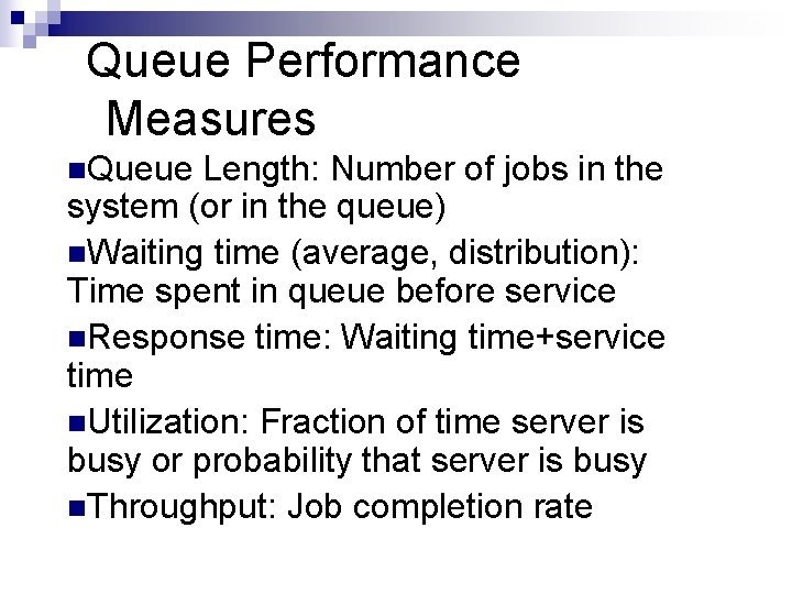
Queue Performance Measures n. Queue Length: Number of jobs in the system (or in the queue) n. Waiting time (average, distribution): Time spent in queue before service n. Response time: Waiting time+service time n. Utilization: Fraction of time server is busy or probability that server is busy n. Throughput: Job completion rate

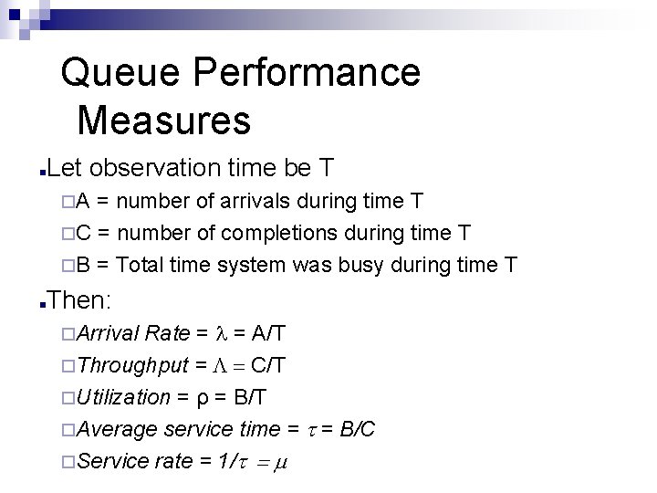
Queue Performance Measures n Let observation time be T ¨A = number of arrivals during time T ¨C = number of completions during time T ¨B = Total time system was busy during time T n Then: Rate = = A/T ¨Throughput = C/T ¨Utilization = ρ = B/T ¨Average service time = = B/C ¨Service rate = 1/ = m ¨Arrival

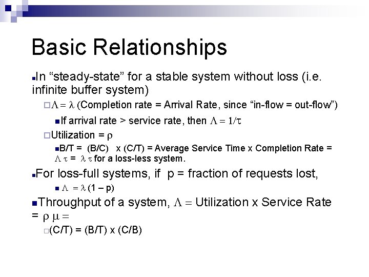
Basic Relationships In “steady-state” for a stable system without loss (i. e. infinite buffer system) n ¨ Completion rate = Arrival Rate, since “in-flow = out-flow”) arrival rate > service rate, then ¨Utilization = n. If n. B/T = (B/C) x (C/T) = Average Service Time x Completion Rate = = for a loss-less system. n For loss-full systems, if p = fraction of requests lost, n (1 – p) n. Throughput = ¨(C/T) of a system, Utilization x Service Rate = (B/T) x (C/B)

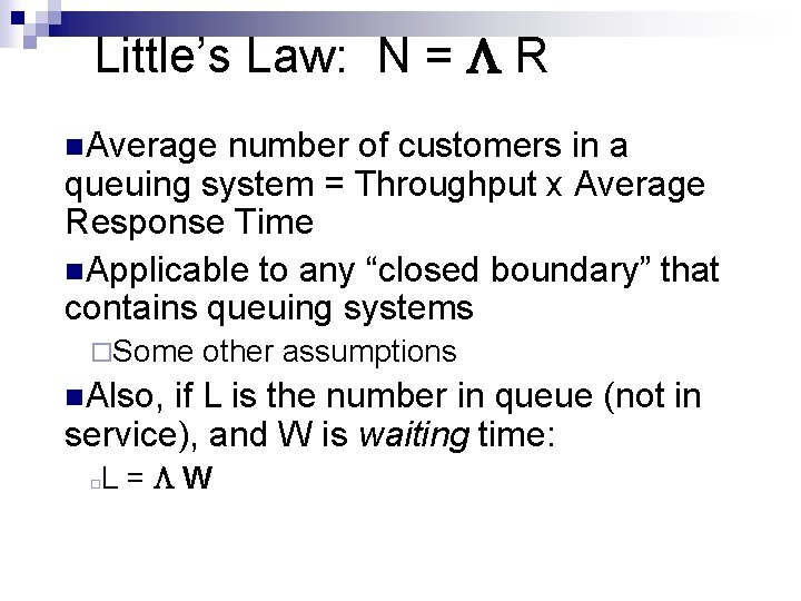
Little’s Law: N = R n. Average number of customers in a queuing system = Throughput x Average Response Time n. Applicable to any “closed boundary” that contains queuing systems ¨Some other assumptions n. Also, if L is the number in queue (not in service), and W is waiting time: L = W ¨

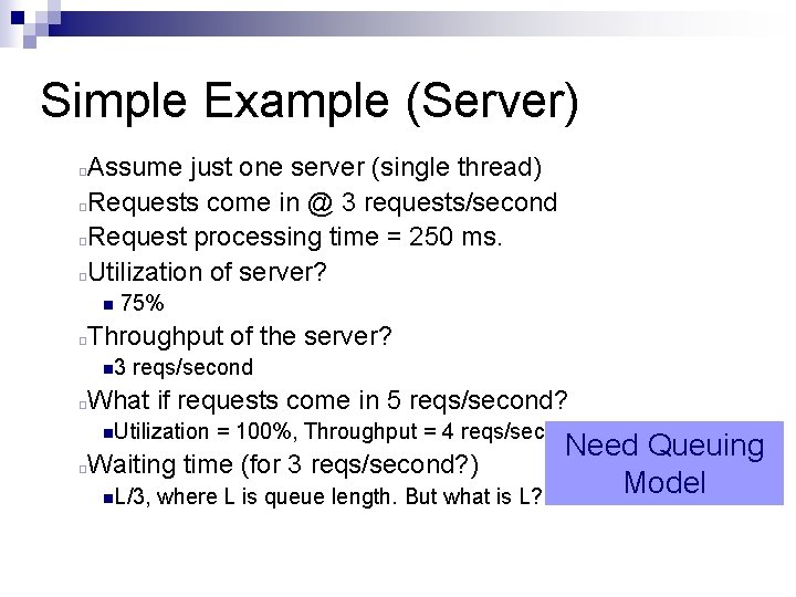
Simple Example (Server) ¨ ¨ Assume just one server (single thread) Requests come in @ 3 requests/second Request processing time = 250 ms. Utilization of server? n ¨ 75% Throughput of the server? n 3 ¨ reqs/second What if requests come in 5 reqs/second? n. Utilization ¨ = 100%, Throughput = 4 reqs/second Waiting time (for 3 reqs/second? ) n. L/3, where L is queue length. But what is L? Need Queuing Model

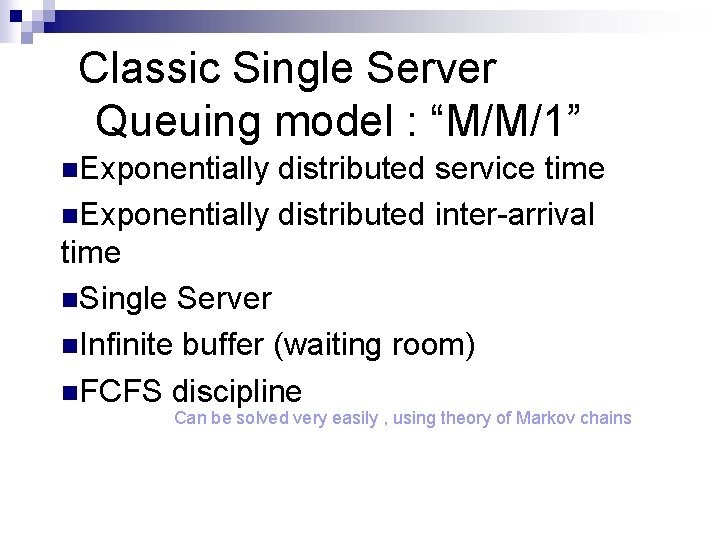
Classic Single Server Queuing model : “M/M/1” n. Exponentially distributed service time n. Exponentially distributed inter-arrival time n. Single Server n. Infinite buffer (waiting room) n. FCFS discipline Can be solved very easily , using theory of Markov chains

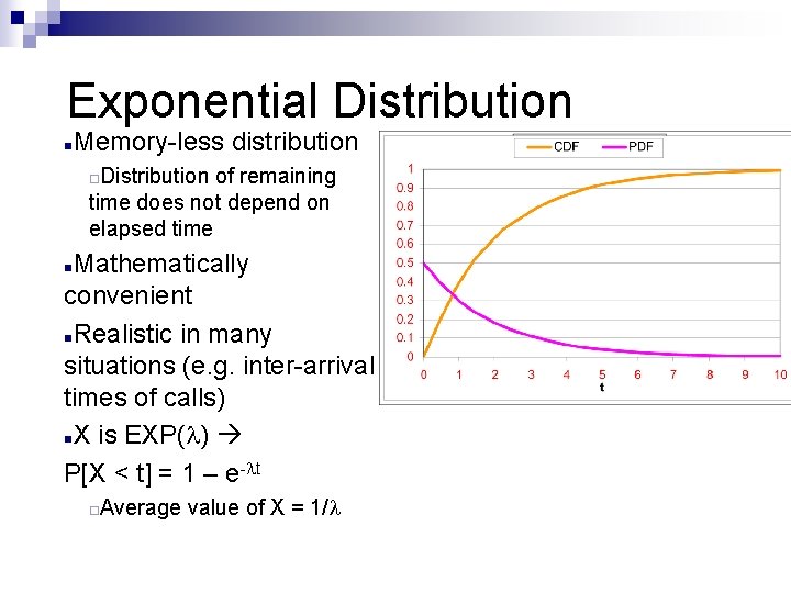
Exponential Distribution n Memory-less distribution Distribution of remaining time does not depend on elapsed time ¨ Mathematically convenient n. Realistic in many situations (e. g. inter-arrival times of calls) n. X is EXP( ) P[X < t] = 1 – e- t n Average value of X = 1/ ¨

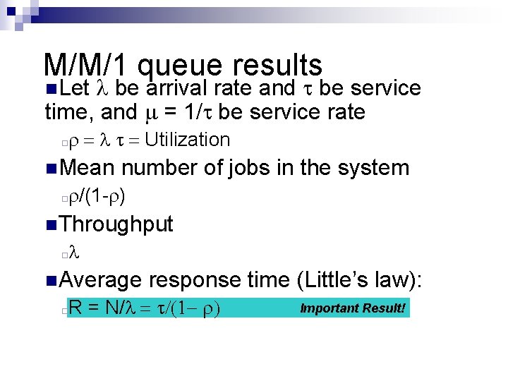
M/M/1 queue results be arrival rate and be service time, and = 1/ be service rate n. Let Utilization ¨ n. Mean number of jobs in the system /(1 - ) ¨ n. Throughput ¨ n. Average response time (Little’s law): R = N/ ¨ Important Result!

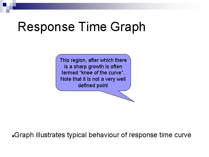
Response Time Graph This region, after which there is a sharp growth is often termed “knee of the curve”. Note that it is not a very well defined point n Graph illustrates typical behaviour of response time curve

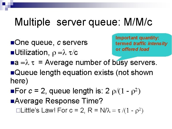
Multiple server queue: M/M/c n. One Important quantity: termed traffic intensity or offered load queue, c servers n. Utilization, c na = Average number of busy servers. n. Queue length equation exists (not shown here) n. For c = 2, queue length is: 2 - n. Average Response Time? ¨Little’s Law! For c = 2, R = N/ -

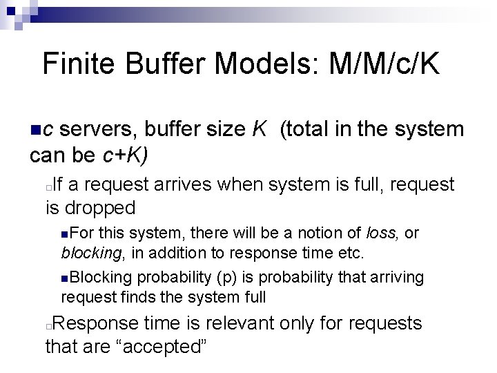
Finite Buffer Models: M/M/c/K nc servers, buffer size K (total in the system can be c+K) If a request arrives when system is full, request is dropped ¨ n. For this system, there will be a notion of loss, or blocking, in addition to response time etc. n. Blocking probability (p) is probability that arriving request finds the system full Response time is relevant only for requests that are “accepted” ¨

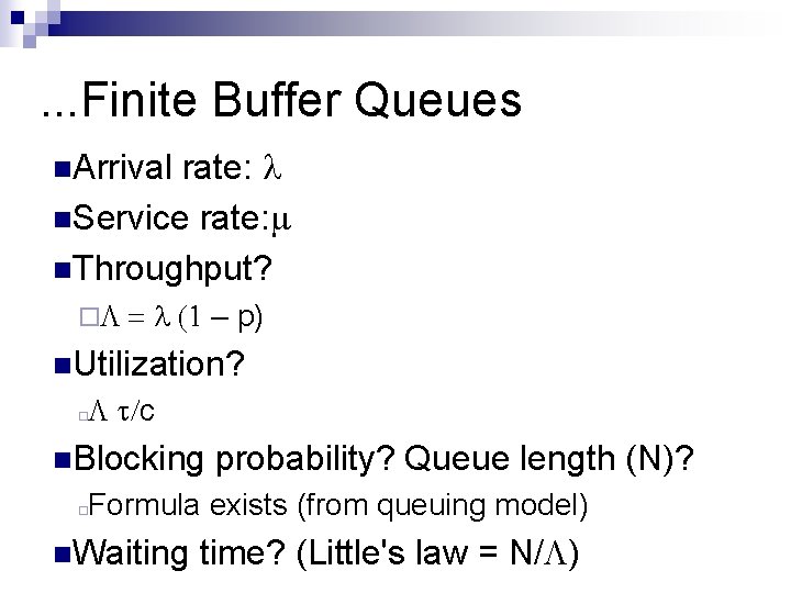
. . . Finite Buffer Queues rate: n. Service rate: n. Throughput? n. Arrival ¨ – p) n. Utilization? c ¨ n. Blocking probability? Queue length (N)? Formula exists (from queuing model) ¨ n. Waiting time? (Little's law = N/ )

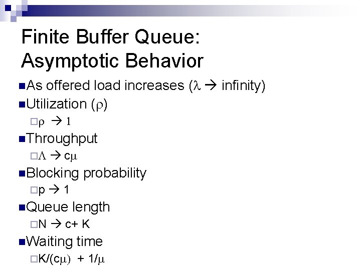
Finite Buffer Queue: Asymptotic Behavior n. As offered load increases ( infinity) n. Utilization ( ) ¨ n. Throughput ¨ c n. Blocking ¨p 1 n. Queue ¨N probability length c+ K n. Waiting time ¨K/(c + 1/

Examples

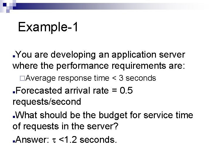
Example-1 You are developing an application server where the performance requirements are: n ¨Average response time < 3 seconds Forecasted arrival rate = 0. 5 requests/second What should be the budget for service time of requests in the server? Answer: <1. 2 seconds. n n n

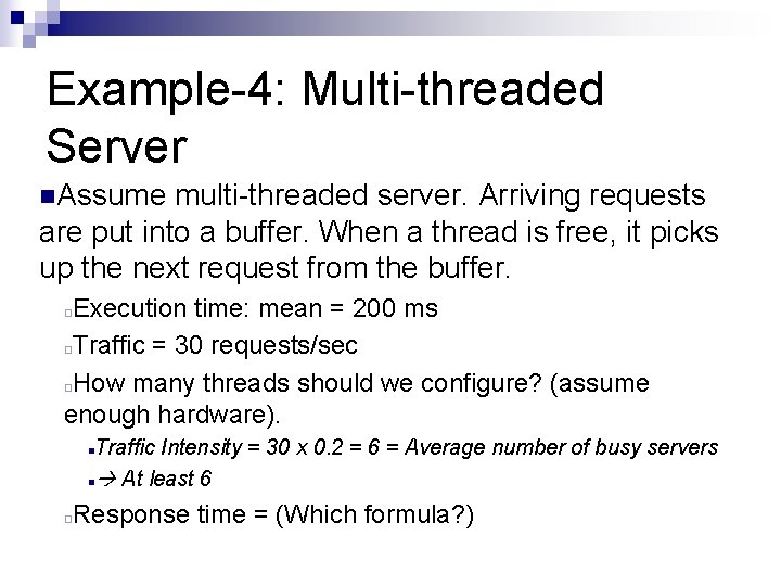
Example-4: Multi-threaded Server n. Assume multi-threaded server. Arriving requests are put into a buffer. When a thread is free, it picks up the next request from the buffer. Execution time: mean = 200 ms Traffic = 30 requests/sec How many threads should we configure? (assume enough hardware). ¨ ¨ ¨ Traffic Intensity = 30 x 0. 2 = 6 = Average number of busy servers At least 6 n n ¨ Response time = (Which formula? )

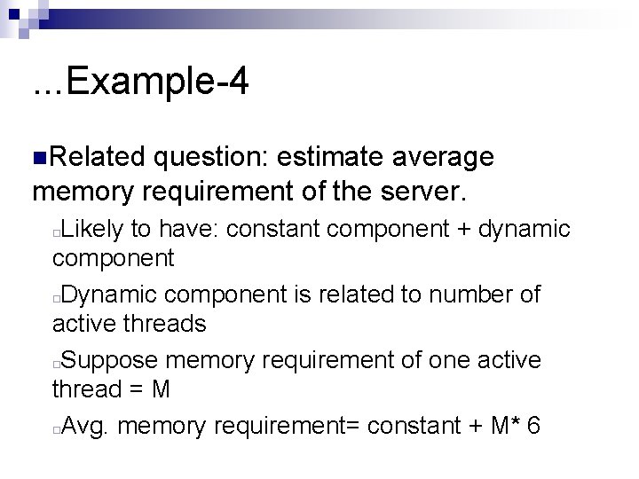
. . . Example-4 n. Related question: estimate average memory requirement of the server. Likely to have: constant component + dynamic component Dynamic component is related to number of active threads Suppose memory requirement of one active thread = M Avg. memory requirement= constant + M* 6 ¨ ¨

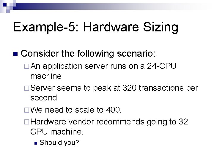
Example-5: Hardware Sizing n Consider the following scenario: ¨ An application server runs on a 24 -CPU machine ¨ Server seems to peak at 320 transactions per second ¨ We need to scale to 400. ¨ Hardware vendor recommends going to 32 CPU machine. n Should you?

Example-5: Hardware Sizing n First do bottleneck analysis! Suppose logs show that at 320 transactions per second, CPU utilization is 67% - What is the problem? What is solution?

Example-5: Hardware Sizing n n Most likely Explanation: Number of threads in server is < number of CPUs Possible diagnosis: ¨ Server has 16 threads configured ¨ Each thread has capacity of 20 transactions per second n n n Total capacity: 320 reqs/second. At this load, 16 threads will be 100% busy average CPU utilization will be 16/24=67% Solution: Increase number of threads – no need for CPUs.

Closed Queuing Systems

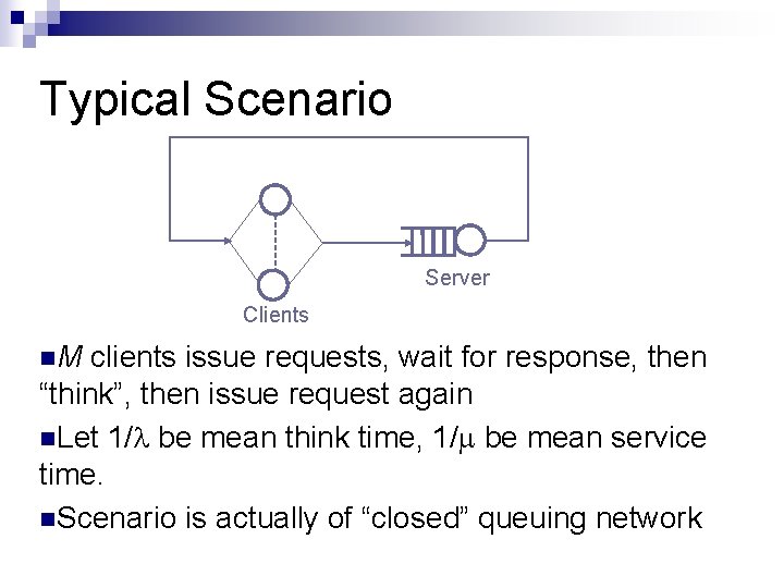
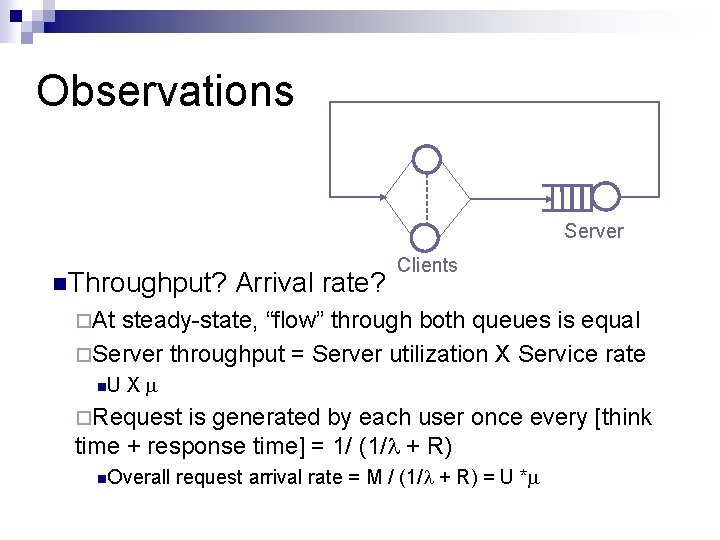
Typical Scenario Server Clients n. M clients issue requests, wait for response, then “think”, then issue request again n. Let 1/ be mean think time, 1/ be mean service time. n. Scenario is actually of “closed” queuing network

Observations Server n. Throughput? Arrival rate? Clients ¨At steady-state, “flow” through both queues is equal ¨Server throughput = Server utilization X Service rate n. U X ¨Request is generated by each user once every [think time + response time] = 1/ (1/ + R) n. Overall request arrival rate = M / (1/ + R) = U *

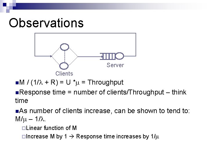
Observations Server Clients n. M / (1/ + R) = U * = Throughput n. Response time = number of clients/Throughput – think time n. As number of clients increase, can be shown to tend to: M/ – 1/. ¨Linear function of M ¨Increase M by 1 Response time increases by 1/

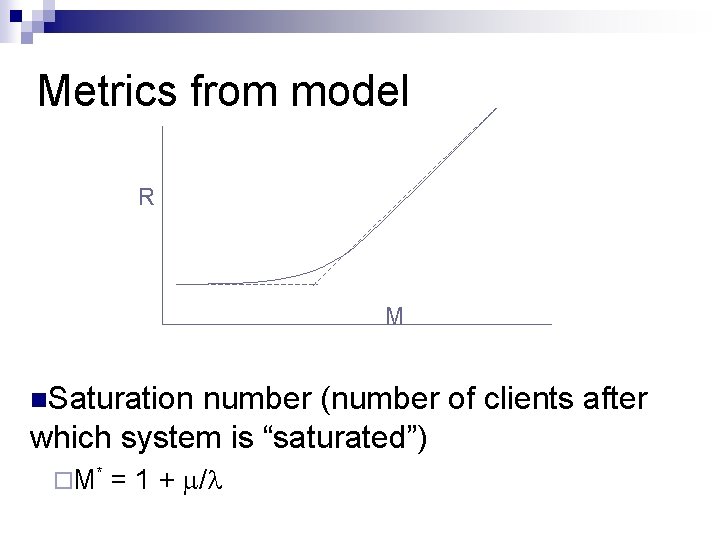
Metrics from model R M n. Saturation number (number of clients after which system is “saturated”) ¨ M* = 1 + /

Queuing networks

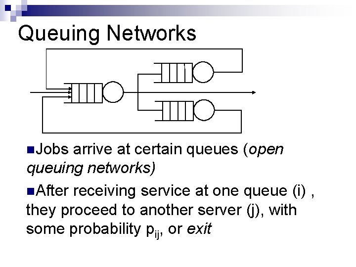
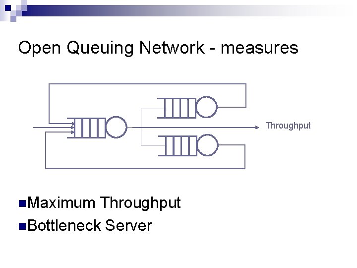
Queuing Networks n. Jobs arrive at certain queues (open queuing networks) n. After receiving service at one queue (i) , they proceed to another server (j), with some probability pij, or exit

Open Queuing Network - measures Throughput n. Maximum Throughput n. Bottleneck Server

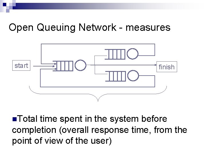
Open Queuing Network - measures start n. Total finish time spent in the system before completion (overall response time, from the point of view of the user)

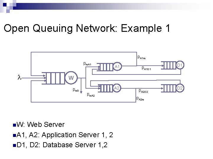
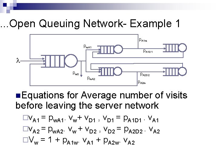
Open Queuing Network: Example 1 p. A 1 w pw. A 1 p. A 1 D 1 W pw 0 n. W: A 1 A 2 pw. A 2 Web Server n. A 1, A 2: Application Server 1, 2 n. D 1, D 2: Database Server 1, 2 p. A 2 D 2 p. A 2 w D 2

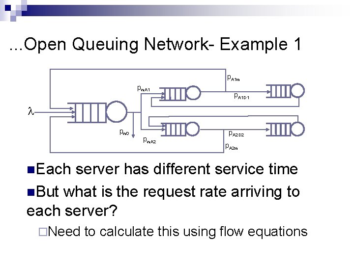
. . . Open Queuing Network- Example 1 p. A 1 w pw. A 1 p. A 1 D 1 pw 0 pw. A 2 p. A 2 D 2 p. A 2 w n. Each server has different service time n. But what is the request rate arriving to each server? ¨Need to calculate this using flow equations

. . . Open Queuing Network- Example 1 p. A 1 w pw. A 1 p. A 1 D 1 pw 0 pw. A 2 p. A 2 D 2 p. A 2 w n. Equations for Average number of visits before leaving the server network ¨v. A 1 = pw. A 1. vw+ v. D 1 , v. D 1 = p. A 1 D 1. v. A 1 ¨v. A 2 = pw. A 2. vw + v. D 2 , v. D 2 = p. A 2 D 2. v. A 2 ¨Vw = 1 + p. A 1 w. v. A 1 + p. A 2 w. v. A 2

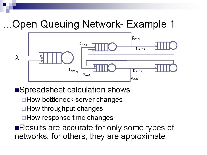
. . . Open Queuing Network- Example 1 p. A 1 w pw. A 1 p. A 1 D 1 pw 0 n. Spreadsheet pw. A 2 p. A 2 D 2 p. A 2 w calculation shows ¨How bottleneck server changes ¨How throughput changes ¨How response time changes n. Results are accurate for only some types of networks, for others, they are approximate