INTERNATIONAL ECONOMICS XU SONG PROFESSOR OF ECONOMICS ANHUI

INTERNATIONAL ECONOMICS XU SONG PROFESSOR OF ECONOMICS ANHUI UNIVERSITY OF FINANCE & ECONOMICS

ANHUI UNIVERSITY OF FINANCE & ECONOMIC Dept. of Int’l Trade and Economics & Business School XU SONG Prof. of Economics Office: 2 nd Floor (West wing), Building 4 Office Hour: Every Afternoon 2: 00－5: 00 Tel: 3128117(O)

1. 1 A Books on International Economics Dominick Salvatore: International Economics 7 th Ed. 2001 Prentice-Hall, Inc. & Tsinghua University Press Paul R. Krugman & Maurice Obstfeld International Economics Theory and Policy 5 th Ed. 2000 Addison Wesley Longman & Tsinghua Uni. Press Dennis R. Appleyard & Alfred J. Field. Jr. . International Economics 4 th ed. 1998 The Mc. Graw-Hill, Inc. & China Machine Press Robert J. Carbaugh: International Economics 6 th ed. 1998 The Mc. Graw-Hill, Inc. & Dongbei Uni. of Finance and Economics Press

Dr. Dominick Salvatore Professor at Fordham University of New York City

1. 1 B Contents of the Book 21 Chapters Part One: International Trade Theory Part Two: International Trade Policies Part Three: Balance of Payments and Exchange Rates Part Four: Open-Economy Macroeconomics and the International Monetary System

1. 1 C Contents of Each Chapter Six Sections in the text Summary ----- 6 paragraphs A Look Ahead--- What is to be discussed in the next chapter. Key Terms Questions for Review----13 Questions Problems---- 13 Problems. Appendix----- More advanced knowledge.

1. 2 A What Is International Economics? It deals with the economic interdependence among nations. It analyzes the flow of goods and services, payments between nations, policies regulating the flow and their effects on national welfare. International trade theory International trade policy International Finance Foreign exchange markets Balance of payments Open economy macroeconomics

1. 2 B International Trade and Policy International trade theory ------- analyzes the basis for and gains from trade (The forces that give rise to trade between nations. List some. ) (Increase in consumption from specialization. ) International trade policy ----examines the reasons for and the effects of trade restrictions and new protectionism. (Tariff, quotas, license, advanced deposits on imports, government procurement, restrictions, technical barrier, environmental barrier, social accountability, ISO …. . . )

1. 2 C International Finance Foreign exchange markets ----- describes the frameworks for the exchange of one national currency for another. We exchange RMB for dollars. Balance of payments ----- measures nation's total receipts from and total payments to the rest of the world. For example, we try to achieve trade balance. Open economy macroeconomics ------ deals with the mechanisms for adjustment in balance of payments disequilibria (国际收支失衡调整机制) as well as the effects of the macroeconomics interdependence (宏观经济 互相依存性) among nations under different international monetary system, and their effects on a nation's welfare.

1. 2 D Purpose to Study International Economics To predict and explain the economic events in the world. To examine the basis for and gains from international trade. To examine the reasons for and the effects of trade restrictions. To understand what is gong in the world and their effects on the world economy. To have a better job!!! Why ? ( Because this knowledge is needed in MNCs, banking and government organizations. )

1. 3 A Assumptions in International Trade • 2× 2× 2 model • No trade restrictions • Perfect mobility of factors within nations and not internationally • Perfect competition Why ? • No transportation costs Answer: It is easier to study international economics. What would happen if we relax these assumptions? Most of our conclusions can still hold. For example, more than 2 nations and more than 2 production factors.

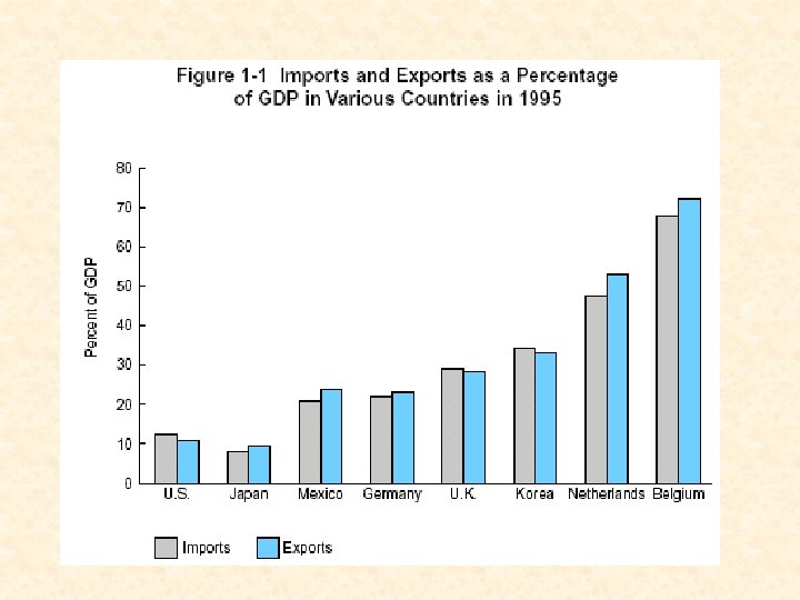
1. 3 B Foreign Trade Dependency What is foreign trade dependency? What is the purpose? How to measure it? -----The ratio of imports and exports of goods and services of a nation to its GDP. What nations have the higher degree of foreign trade dependency? What is the trade dependency in China? Why is it like this? Why is international trade very important to a nation? A nation can not survive without foreign trade, such as Japan, Germany, Belgium and others. A nation can not produce all the products it needs, for example that US can not produce coffee, cocoa, tea, scotch and other products, they don't have the materials. The economies of all nations are closely related to each other. To improve the standard of living.

1. 4 A China GDP and Foreign Trade Dependency Year GDP (bill. ￥) Exp+Imp (bill. $) Exp+Imp GDP 1997 7477. 2 325. 16 36. 0% 182. 79 20. 3% 142. 37 15. 7% +404. 2 1998 7834. 5 323. 95 33. 7% 183. 71 19. 1% 140. 24 14. 6% +434. 2 1999 8206. 7 360. 63 36. 4% 194. 93 19. 7% 165. 70 16. 7% +292. 3 2000 8944. 2 474. 30 44. 0% 249. 20 23. 0% 225. 09 21. 0% +241. 1 2001 9593. 3 509. 77 45. 0% 266. 15 24. 0% 243. 61 21. 0% +225. 4 2002 10239. 8 620. 80 50. 3% 325. 57 26. 4% 295. 22 23. 9% +303. 5 2003 851. 21 2004 Data source: China Customs Export (bill. $) 438. 37 Export GDP Import (bill. $) 412. 84 Import GDP Balance ($) +255. 4

1. 4 B Reasons for the High Dependency GDP is smaller than it should be. Many values created are not included in the GDP. For example, the pigs, cattle and some others in the countryside are not included. The real GDP is much higher, three times higher than it is. Processed products take up too much percentage in the exports. In the last several years, the value of processed goods is more than 50% in the exports. RMB was depreciating all the years before 1994. In 1984, the exchange rate was US$1. 00 for ￥ 2. 32. In 1990, it was USD 1. 00 for ￥ 4. 72. In 1994, USD 1. 00 for ￥ 8. 62. What will happen in the future to China trade dependency ?

1. 4 C Foreign Trade Dependency in Some Nations 1970 1980 1993 Developing countries India 3. 5 5. 0 6. 0 8. 6 Indonesia 11. 5 28. 1 24. 2 23. 2 Korea 9. 3 27. 5 25. 6 24. 8 Pakistan 4. 0 11. 1 14. 0 12. 9 Tailand 10. 0 20. 1 26. 9 29. 5 Advanced countries Japan 9. 5 12. 3 9. 8 8. 6 Canada 19. 8 25. 7 22. 5 26. 6 America 4. 2 8. 3 7. 2 7. 4 France 12. 5 17. 6 16. 5 Germany 18. 6 23. 8 27. 4 19. 9 Italy 12. 3 17. 3 15. 6 16. 9 United Kingdom 15. 7 20. 5 19. 0 19. 3 Australia 12. 1 13. 7 13. 3 14. 8

1. 5 A Basic International Trade Data

1. 5 A Basic International Trade Data(2)

1. 5 A Basic International Trade Data(3)

1. 5 A Basic International Trade Data(4)

1. 5 A Basic International Trade Data(5)

1. 6 Some Questions 1. Import/GDP has _______in recent years. (risen, fallen, remained steady) (From 15. 7 % in 1997 to 23. 9 % in 2002. ) 2. Export/GDP has _______in recent years. (risen, fallen, remained steady) (From 20 % in 1997 to 26. 4 % in 2002. ) 3. Which nation is our largest trading partner? ( Japan: 133. 57 billion dollars in 2003 ) 4. Which is the second largest trading partner? ( U. S. 126. 33 billion dollars in 2003 )

1. 6 Some Questions (2) 1. The purpose of trade is to_______. a. improve consume well-being. b. create jobs. 2. Work is a ____. a. cost b. benefit 3. Exports are ____. a. cost b. benefit 4. The objective of international trade is to _____. a. get goods cheaply b. create jobs 5. NAFTA has had a greatest impact on the _____ of U. S. b. unemployment a. inflation rate ( All of “a” are correct. They are consistent with standard economic theory. All of “b” are wrong, but they are consistent with old economic theory. ) International economics is not always what you think it is!!! 1. People trade to improve their well-being. Creating jobs is a means to an end. 2. Would you like to work for free? 3. Exports: you make it but don’t consume it. 4. Trade is great at cost-cutting but no net impact on jobs. 5. NAFTA reduces goods prices.

Chapter 2 The Law of Comparative Advantage

2. 1 Introduction In this chapter, we will examine the development of trade theory from the 17 th century to the first half of the 20 th century. This historical approach is useful not because we are interested in the history of economic thoughts but because it is a convenient way of introducing the concepts and theories of international trade from the simple to the most complex and realistic. We will use 2 X 2 X 1 model and start from absolute advantage, to comparative advantage and to opportunity costs and production possibility frontiers.

2. 2 Mercantilists’ Views on Trade Mercantilism ---- Some people wrote articles on international trade. Their philosophy was known as mercantilism. Representative ----- Thomas Munn (1571 -1641) Works ---- England’s Treasure by Foreign Trade Wealth: The way for a nation to become rich and powerful was to export more than it imported. The resulting surplus would then be settled by an inflow of bullion. The more gold and silver a nation had, the richer and more powerful it was. What kind of policy should be adopted? The government had to do all in its power to stimulate the nation’s exports and discourage and restrict imports. What is the nature of the trade? One nation could gain only at the expense of other nations. It is called a zero-sum game.

2. 2 b Different Views on National Wealth Mercantilists attached importance to bullion. But today we pay attention to the stock of human resources, man-made and natural resources available for producing goods and services. The greater this stock of useful resources, the greater is the inflow of goods and services to satisfy human wants and the higher the standard of living in the nation.

2. 2 c Purposes of Mercantilists’ Trade Theory To maintain larger and better armies with more gold and silver and consolidate their power at home; To acquire more colonies with improved armies and navies; To do more business with more money; To stimulate national output, develop national economy and increase employment.

2. 3 Adam Smith’s Trade Theory The basis for trade ------ Absolute advantage If one nation is more efficient than another nation in the production of one commodity, the nation has absolute advantage in that commodity. The pattern of trade ------- both nations can gain by each specializing in the production of the commodity of its absolute advantage and exporting part of its output with the other nation for the commodity of its absolute disadvantage. Policy: Free trade policy should be adopted to make better use of resources and maximize world welfare.

2. 3 b Where Do the Gains Come From? By specialization, resources are utilized in the most efficient way and the output of both commodities will rise. The increased output measures the gains from specialization in production available to be divided between the two nations through trade.

2. 3 d Difference Between Mercantilists & Adam Smith According to mercantilists’ view, one nation could only gain at the expense of another nation and each government should take strict control of all economic activities and trade. They should adopt protectionist measures to stimulate exports and restrict imports. But according to Adam Smith, all nations could gain from free trade and each nation should adopt a laissez-faire policy (free trade policy).

2. 3 e Illustration of Absolute Advantage U. S. U. K. Wheat(bushels/man-hour) 6 1 Cloth(yards/man-hour) 4 5 U. S. has greater efficiency in production of wheat (absolute advantage) and it should specialize in the production of wheat and exchange for cloth , while U. K. has greater efficiency in production of cloth and it should specialize in the production of cloth and exchange for wheat (absolute advantage). What happens if U. S. exchanges 6 W for 6 C with U. K. ?

2. 3 f Comments on the Absolute Advantage It can only explain small part of world trade today, but it can not explain most of the trade between the developed and the developing countries. Can we use theory to carry out foreign trade? It can not even explain the trade between advanced countries because their productivities are almost the same.

2. 4 a The Law of Comparative Advantage Representative ----- David Ricardo (1772 -1823) Works ---- Principles of Political Economy and Taxation It explains how mutually beneficial trade can take place even when one nation is less efficient than ( has an absolute disadvantage) the other nation in the production of all commodities. The less efficient nation should specialize in and export the commodity in which its absolute disadvantage is smaller (this is the commodity of its comparative advantage), and should import the other commodity.

2. 4 b Illustration of Comparative Advantage U. S. U. K. Wheat(bushels/man-hour) 6 1 Cloth(yards/man-hour) 4 2 What should U. S. or U. K. produce? At what rate should they exchange their commodities?

2. 4 c Gains from Trade Rate of Exchange U. S. Gains UK Gains 6 W: 4 C 0 C 8 C 6 W: 6 C 2 C 6 C 6 W: 8 C 4 C 4 C 6 W: 10 C 6 C 2 C 6 W: 12 C 8 C 0 C Trade range: 4 C<6 W<12 C Conclusion: The closer the rate of exchange is to 4 C=6 W, the smaller is the share of the gain going to the United States and the larger is the share of the gain going to the United Kingdom. On the other hand, the closer the rate of exchange is to 6 W=12 C, the greater is the gain of the United States relative to that of the United Kingdom.

2. 4 d Exception to Law of Comparative Advantage U. S. U. K. Wheat(bushels/man-hour) 6 3 Cloth(yards/man-hour) 4 2 Even if one nation has an absolute disadvantage with respect to the other nation in the production of both commodities, there is still a basis for mutually beneficial trade, unless the absolute disadvantage is in the same proportion for the two commodities. This kind of exception is rare.

2. 4 e How Can They Trade? How can they trade if one nation is in absolute disadvantage in the production of both commodities? They can still trade when the wage is sufficiently lower in one nation than it is in the other nation and when both commodities are expressed in terms of the same currency. U. S. U. K. Wheat(bushels/man-hour) 6 1 Cloth(yards/man-hour) 4 2 Exchange rate: ￡ 1. 00=$2. 00 Unit Price of Wheat Unit Price of Cloth $6 per hour in U. S. , U. S. $1. 00 $1. 50 ￡ 1 per hr in U. K. , U. K. $2. 00 $1. 00

2. 4 f Price of Wheat and Cloth in U. S. & U. K. Exchange rate: ￡ 1. 00=$1. 00 Unit Price of Wheat Unit Price of Cloth U. S. $1. 00 $1. 50 U. K. $1. 00 $0. 50 U. S. cannot export wheat to U. K. But U. K. can continue to export cloth to U. S. The trade will become unbalanced. The dollar price of pound will have to rise to ￡ 1. 00=$2. 00, instead of ￡ 1. 00=$1. 00. Exchange rate: ￡ 1. 00=$3. 00 U. S. U. K. Unit Price of Wheat $1. 00 $3. 00 Unit Price of Cloth $1. 50 U. K. can’t export cloth to U. S. But U. S. can continue to export wheat to U. K. The trade becomes unbalanced. The dollar price of pound has to fall to ￡ 1. 00=$2. 00, instead of ￡ 1. 00=$3. 00.

2. 5 Assumptions for Comparative Advantage 2× 2 model-----Two nations, two commodities and one factor Free trade. Perfect mobility of labor within each nation but immobility between the two nations. Constant costs of production. No transportation costs No technical change The labor theory of value.

2. 5 b The Opportunity Cost Theory It is the amount of a second commodity that must be given up in order to release enough resources to produce one additional unit of the first commodity (comp. cost stresses the opportunity cost). The nation with lower opportunity cost in the production of a commodity has a comparative advantage in that commodity and a comparative disadvantage in the second commodity. Opportunity Costs of Wheat in Terms of Cloth 1 W 2/3 C 1 W 2 C Opportunity Costs of Cloth in Terms of Wheat 3/2 W 1 C 1/2 W 1 C

2. 5 c Production Possibility Frontier It is a curve showing the various alternative combinations of two commodities that a nation can produce by fully utilizing all of its resources with the best technology available to it.

2. 5 d Production Possibility Schedules for Wheat and Cloth in U. S. & U. K.

2. 5 e PPF in U. S & U. K

2. 5 f Features of PPF Each point on a frontier represents one combination of wheat and cloth that the nation can produce. Points inside the PPF are possible, but are inefficient. It means that the nation has some idle resources or it is not using the best technology available to it. Points outside the PPF are not possible because the nation does not have enough resources to produce at those points. The downward slope of the PPF indicates that when it wants to increase the production of the first commodity, it has to give up the second commodity The straight line reflects the fact that the opportunity cost is constant----constant opportunity costs.

2. 5 g Constant Opportunity Costs It means that the constant amount of a commodity must be given up to produce each additional unit of another commodity. We have constant opportunity cost when (1) resources or factors are either perfect substitutes for each other or used in fixed proportion in the production of both commodities; (2) all units of the same factor are homogeneous or exactly the same quality.

2. 5 h Consumption Frontier It shows the combination of consumption that the nation actually chooses to consume. In the absence of trade, the production possibility frontier is also the consumption frontier.

2. 6 Basis for and Gains from Trade under Constant Costs Before trade: U. S. produces at Point A and consumes at point A( 90 W and 60 C); U. K. produces at Point A’ and consumes at point A’(40 W and 40 C). Total output & consumption: Wheat=90 W+40 W=130 W Cloth=60 C+40 C=100 C With trade: U. S. produces at Point B (180 W), exchanges 70 W for 70 C with U. K. and consumes 110 W & 70 C (gain 20 W and 10 C) ; U. K. produces at Point B’(120 C), exchanges 70 C for 70 W with U. S. and consumes 70 W & 50 C (gain 30 W and 10 C). Total consumption: Wheat=110 W+70 W=180 W Cloth=70 C+50 C=120 C

2. 6 b Relative Prices and Comparative Advantage It is the price of one commodity divided by the price of another commodity. This equals the opportunity cost of the commodity and is given by the absolute slope of the production possibility frontier (sometimes it is called marginal rate of transformation). Relative Price of Wheat: PW/ PC =2/3 in U. S. , Pw/ Pc =2/1 in U. K. Relative Price of Cloth: PC/ Pw =1. 5 in U. S. , Pc/ Pw =0. 5 in U. K. A nation has a comparative advantage if the relative price of a commodity is lower than that in the other nation. Opportunity Cost = Relative Price＝MRT

2. 6 c Equilibrium Relative Commodity Prices With D & S At PW /PC =2/3, U. S. Produces 180 W; At PW /PC =2, U. K. produces 60 W. At PC /PW =1/2, U. K. produces 120 C; at PC /PW =3/2, U. S. produces 120 C.

2. 6 d Large Country and Small Country Large country is a country that its trade can influence the world price. Small country is country that its trade can not affect the world supply and demand. Small country case is the situation where trade takes place at the pretrade-relative commodity prices in the large nation so that the small nation receives all of the benefits from trade.

2. 7 Empirical Test of Ricardian Trade Model The first empirical test of the Ricardian trade model was conducted by Mac. Dougall in 1951 and 1952 using 1937 data. The results indicated that those industries where labor productivity was relatively higher in the United States than in the United Kingdom were the industries with the higher ratios of U. S. to U. K. exports to third markets. These results were confirmed by Balassa using 1950 data, Stern using 1950 and 1959 data, and Golub using 1990 data. Thus, it can be seen that comparative advantage seems to be based on a difference in labor productivity or costs, as postulated by Ricardo. However, the Ricardian model explains neither the reason for the difference in labor productivity or costs across nations nor the effect of international trade on the earnings of factors.

2. 7 b Labor Productivity and Comparative Advantage

2. 7 c Comments on Comparative Advantage Ricardian trade model has to a large extent been empirically verified, but it has a serious shortcoming in that it assumes rather than explains comparative advantage. That is, Ricardo in general provided no explanation for the difference in labor productivity and comparative advantage between nations and they could not say much about the effect of international trade on the earnings of factors of production. These were left for Heckscher-Ohlin model.

2. 8 Problems

A 2. 1 Comparative Ad with More Than Two Commodities Commodity Price in U. S. Price in U. K. $ price in U. K. A B C D E $ ￡ ￡ 1=$2 $2 $4 $6 $8 $10 ￡ 6 ￡ 4 ￡ 3 ￡ 2 ￡ 1 $12 $8 $6 $4 $2 ￡ 1=$1 $6 $4 $3 $2 $1 ￡ 1=$3 $18 $12 $9 $6 $3 What is the dollar price of pound for US to export at least one commodity? ￡ 6. 00> $2. 00, ￡ 1. 00 > $0. 33 What is the dollar price of pound for UK to export at least one commodity? ￡ 1. 00< $10. 00 Range of Exchange Rate: $0. 33 < ￡ 1. 00 <$10

A 2. 2 Comparative Ad with More Than Two Nations What is the range of Pw/Pc if there is trade between the nations? Range of Pw/Pc: 1<Pw/Pc <5 What would happen if Pw/Pc =3, Pw/Pc=4 and 2?

Chapter 3 The Standard Theory of International Trade

3. 1 Introduction This chapter will extend our simple model to the more realistic case of increasing opportunity costs. Tastes or demand preferences are introduced with community indifference curves. We then will see how these forces of supply and demand determine the equilibrium relative commodity price in each nation in the absence of trade under increasing opportunity costs.

3. 1 b Review What is opportunity cost? And constant opportunity cost? Under what condition can we have constant opportunity cost? What is production possibility frontier? What does the production possibility frontier look like with a constant opportunity cost?

3. 2 a Increasing Opportunity Costs The increasing amounts of one commodity that a nation must give up to release just enough resources to produce each additional unit of another commodity. This is reflected in a production frontier that is concave from the origin (rather than a straight line). ? 1. Resources or factors of production are not homogeneous. It means that as the nation produces more of a commodity, it must utilize resources that become progressively less efficient or less suited for the production of that commodity. As a result, the nation must give up more and more of the second commodity to release just enough resources to produce each additional unit of the first commodity. 2. They are not used in the same fixed proportion or intensity on the production of all commodities.

3. 2 a The Increasing Opportunity Costs(B) Concave PPF reflect increasing opportunity costs in each nation in the production of both commodities. Nation 1 must give up more and more Y for each additional batch of 20 X that it produces. This is illustrated by downward arrows of increasing length. Similarly, Nation 2 incurs increasing opportunity costs in terms of forgone X for each additional batch of 20 Y it produces.

3. 2 b Determinants of Different Shape of PPF What determine the shape of production possibility frontiers? Production possibility frontiers are different because the two nations have different factor endowments or resources at their disposal or they use different technologies in production. Can they change? As the supply of factors or technologies changes over time, a nation’s production possibility frontier may also change, such as the production frontiers in Japan in 1950 s and 1990 s. China production possibility frontier will also change.

3. 2 c Marginal Rate of Transformation (MRT) Marginal rate of transformation (MRT) is the amount of one commodity that a nation must give up to produce each additional unit of another commodity. It is another name for the opportunity cost of a commodity and is given by the slope of the production frontier at the point of production. The marginal rate of transformation of X for Y refers to the amount of Y that a nation must give up to produce each additional unit of X. Thus, MRT is another name for the opportunity cost of X and is given by the slope of the production frontier at the point of production. If the slope of the production frontier of Nation 1 at point A is 1/4, it means that Nation 1 must give up 1/4 of a unit of Y to release enough resources to produce one additional unit of X at this point.

3. 3 a Community Indifference Curve It shows the various combinations of two commodities that yield equal satisfaction to the community or nation. Higher curves refer to greater satisfaction; Lower curves refer to less satisfaction. Negatively sloped and convex from the origin, Not cross each other.

3. 3 b Marginal Rate of Substitution The MRS of X for Y in consumption refers to the amount of Y that a nation could give up for one extra unit of X and still remain on the same indifference curve. This is given by the absolute slope of the community indifference curve at the point of consumption and declines as the nation moves down the curve. For example, the slope of indifference curve I is greater at point N than at Point A. The declining MRS shows that the more of X and less of Y a nation consumes, the more valuable to the nation is a unit of Y at the margin compared with a unit of X. Therefore, the nation can give up less and less Y for each additional unit of X it wants. Comparison: While increasing opportunity cost in production is reflected in concave production frontier, a declining MRS in consumption is reflected in convex community indifference curves.

3. 3 c Difficulties with Community Indifference Curves A set of community indifference curves reflect a particular income distribution in the nation. A different income distribution would result in a completely new set of indifference curves. The new curve may intersect the previous indifference curve. This happens as a nation opens trade or increase its volume of trade. Exporters benefit but domestic producers competing with imports will suffer. There is also differential impact on consumers. Trade will change the distribution of real income in the nation and may cause indifference curves to intersect. Compensation Principle: ---- the nation will benefit from trade How to solve it? if the gainer would be better off even after fully compensating the losers for their losses. The government can compensate the losers through transfer payment, tax, subsidies and other means.

3. 4 Equilibrium In Isolation In isolation, a nation is in equilibrium when it reaches the highest indifference curve possible given its production frontier. It is at the point where a CIC is tangent to the nation’s PPF. The common slope of the two curves at the tangency point gives the internal equilibrium relative commodity price (equilibrium point in isolation) and reflects the nation’s comparative advantage. The tangency point can be on lower indifference curves, but it would not maximize the nation’s welfare; on higher curves, the nation would not achieve the level of welfare with the existing resources and technologies.

3. 4 b Equilibrium In Isolation

3. 4 c Equilibrium-Relative Commodity Price in Isolation The equilibrium relative commodity price in isolation is a price at which a nation is maximizing its welfare in isolation. It is given by the slope of the common tangent to the nation's PPF and CIC at the autarky point of production and consumption. Since in isolation PA< PA’, nation 1 has a comparative advantage in commodity X, and nation 2 in Y. The equilibrium relative commodity prices in each nation in autarky are determined by the forces of supply (as given by the nation’s production possibility frontiers) and the forces of demand (given by the nation’s indifference map) in each nation. Under increasing costs: If indifference curve is of a different shape, it would be tangent to the production frontier at a different point and determine a different relative price of X in Nation 1. Under constant cost: The equilibrium Px/Py is constant regardless of the level of output and demand is given by the constant slope of the production frontier.

3. 5 Basis for & the Gains from Trade with Increasing Costs The basis for mutually beneficial trade is the relative commodity price. A difference in the relative commodity prices between the two nations reflects their comparative advantage. The nation with lower relative price for a commodity has a comparative advantage in that commodity. The pattern: Each nation should specialize in the production of the commodity of its comparative advantage and exchange part of its output with the other nation for the commodity of its comparative disadvantage. Specialization incurs increasing opportunity costs and it will continue until relative commodity prices in the two nations become equal at the level at which trade is in equilibrium. Through trading, both nations will end up consuming more products than in the absence of trade.

3. 5 b Illustrations of the Basis for and Gains

3. 5 c Equilibrium-Relative Commodity Price It is the common relative commodity price in two nations at which trade is balanced. At this relative price, the amount of X that nation 1 exports equals the amount of X that nation 2 imports. The amount of Y that nation 2 exports matches the amount of Y that nation 1 imports. At other relative price, trade cannot persist because it becomes unbalanced. The greater is Nation 1’s desire for Y(the commodity exported by Nation 2) and the weaker is Nation 2’s desire for X (the commodity exported by Nation 1), the closer the equilibrium price with trade will be to the pretrade equilibrium price in Nation 1 and smaller will be nation 1’s share of the gains. If the pretrade relative price were the same in both nations, there would be no comparative advantage or disadvantage in either nation and no specialization in production or mutually beneficial trade would take place.

3. 5 d Complete and Incomplete Specialization Under constant opportunity costs, both nations specialize completely in the production of the commodity of their comparative advantage. Under increasing opportunity costs, both nations have incomplete specialization in the production of the commodity of their comparative advantage. The reason is -----increasing opportunity cost!!! Specialization incurs increasing opportunity cost. The relative commodity price move toward each other until they are identical in both nations. Nation 1 specializes in the production of X, it incurs increasing opportunity costs in producing X. The same is true for nation 2.

3. 5 e Small Country Case with Increasing Costs Under constant opportunity costs, the only exception to complete specialization in production was in the small country case. The large nation continued to produce both commodities even with trade, because the small nation could not satisfy all of the demand for imports of the large nation. Under increasing opportunity costs, both nations have incomplete specialization in the production of the commodity of their comparative advantage, even if it is the small nation. The equilibrium relative price of X in the world market is 1 (Pw=1), and it is not affected by trade with small Nation 1. In absence of trade, the relative price of X in Nation 1 (PA=1/4) is lower than the world market price, Nation 1 has a comparative advantage in X. With trade, Nation 1 specializes in X until it reaches point B on the production frontier, where PB=1=Pw. Nation 1 does not specialize completely in the production of X.

3. 5 f The Gains from Exchange & Specialization

3. 6 Trade Based on Difference in Taste If the production possibility frontiers are identical, is there any basis for trade? Yes. The basis for trade is the difference in tastes or demands. The nation with a smaller demand for a commodity will have a lower autarky relative price for, and a comparative advantage in the commodity. Assumptions: Identical production frontiers in the two nations.

3. 6 Illustration of Trade Based on Different Taste

A 3. 1 Appendix to CH 3 Isoquants, isocosts and equilibrium Illustrations of these concepts for 2 nations, commodities and 2 factors Edgeworth box diagram and the production frontier Change in the ratio of resource use in the specialization

A 3. 2 a Isoquant It is a curve showing the various combinations of 2 factors (K and L) that a firm can use to produce a specific level of output. It has the same general characteristics as indifference curves. Higher isoquants refer to larger outputs and lower ones refer to smaller outputs. They are negatively sloped because a firm using less K must use more L to remain on the same isoquants. The absolute slope of the isoquant is called the marginal rate of technical substitution of labor for capital in production (MRTS) and measures how much K the firm can give up by increasing L by one unit and still remain on the same isoquant. As a firm moves down an isoquant and uses more L and less K, it finds it more and more difficult to replace K with L. MRTS is diminishing. It makes the isoquant convex from the origin. They do not cross because an intersection means the same level of output on the two isoquants.

A 3. 2 b Illustration of Isoquant

A 3. 3 Isocost is a line showing the various combinations of two inputs (K, L) that a firm can hire for a given expenditure at given factor prices. If the total expenditure is $30 and PK=$10 and PL=$5, how to allocate it? 3 K or 6 L can be used in production or other combination. The absolute slope of the isocost of 3/6=1/2 gives the relative price of L, that is PL/PK =$5/$10 =1/2

A 3. 4 Equilibrium and Expansion Path When a producer maximizes output for a given cost outlay, that is, reaching the highest isoquant possible with a given isocost, he is in equilibrium. When an isoquant is tangent to an isocost (MRTS= PL/PK) we have equilibrium. Expansion path is the straight line from the origin connecting equilibrium points, such as A 1 and A 2. A production function shows that increasing inputs in a given proportion results in output increasing in the same proportion. Q= f (K, L)

A 3. 5 a Isoquants, isocosts and equilibrium Isoquants 1 X and 2 X give the various combinations of K and L that the firm can use to produce one and two units of X, respectively. Isocosts are the lines from 3 K to 6 L and from 6 K to 12 L, the absolute slope measures the PL /PK =1/2. Equilibrium is at points A 1 and A 2, the highest isoquants possible for a given total expenditure. The expansion path gives the constant K/L=1/4 ratio in producing X.

A 3. 5 b Production with Two Nations, Two Commodities and Two Factors Y is the K-intensive commodity in both nations. The K/L ratio is lower in Nation 1 than in Nation 2 in both X and Y because PL/PK is lower in Nation 1. Since Y is always the K-intensive and X is always the L-intensive commodity in both nations, the X and Y isoquants intersect only once in each nation(discussed in CH 5).

A 3. 6 Edgeworth Box and Production Frontier for Nation 1

A 3. 7 Edgeworth Box and Production Frontier for Nation 2

A 3. 8 Some Important Conclusions The movement from point A to point B on Nation 1's contract curve refers to an increase in the production of X (the commodity of its comparative advantage) and results in a rise in the K/L ratio. This rise in the K/L ratio is measured by the increase in the slope of a straight line (not drawn) from origin Qx to point B as opposed to point A. The same movement from point A to point B also raises the K/L ratio in the production of Y. This is measured by the increase in the slope of a line from origin Oy to point B as opposed to point A. The rise in the K/L ratio in the production of both commodities in Nation 1 can be explained as follows. Since Y is K intensive, as Nation 1 reduces its output of Y, capital and labor are released in a ratio that exceeds the K/L ratio used in expanding the production of X. There would then be a tendency for some of the nation's capital to be unemployed, causing the relative price of K to fall (i. e. , PL/PK to rise). Nation 1 substitutes K for L in the production of both commodities until all available K is once again fully utilized. Thus, the K/L ratio in Nation 1 rises in the production of both commodities. This also explains why the production contract curve is not a straight line but becomes steeper as Nation 1 produces more X ( it moves farther from Ox). The contract curve would be a straight line only if relative factor prices remained unchanged, and here factor prices change.