International Baccalaureate Higher Level International Baccalaureate Higher Level

International Baccalaureate Higher Level International Baccalaureate Higher Level International Baccalaureate Higher Level International Baccalaureate Higher Level International Baccalaureate Higher Learning outcomes Level International Baccalaureate Higher Level International This International work will help. Baccalaureate you Baccalaureate Higher Level International Baccalaureate Higher Level 1. Perform a goodness of. Level fit test. International Baccalaureate Higher Level 2. Perform a test for independence on. International contingency. Baccalaureate Higher Leveltables International Baccalaureate Higher Level International Baccalaureate Higher Level International Baccalaureate Higher Level International Baccalaureate Higher Level International Baccalaureate The Chi-Squared Test

The Chi-squared Distribution The distribution has one parameter v, pronounced ‘new’ and a constant , and the shape of the distribution is given by the probability distribution function (p. d. f. ) where If X is distributed in this way we write The p. d. f. is very complicated and is not required for the IB course, but the shape of its graph is shown below.

Some features of the distribution are • It is reversed J-shaped for v = 1 and v = 2 • it is positively skewed for v > 2. • The larger the value of v, the more symmetrical the distribution becomes. • When v is large, the distribution becomes approximately normal.

The Significance Test There are two tests A test for independence or for association. This is conducted if you have some practical data with two variables and you want to know if they are independent or there is an association between them. We make two hypothesis, the null hypothesis H 0, is that the factors are independent and the alternate hypothesis H 1, is that they are not. A goodness of fit test. This is used if you have some practical data and you want to know how well it fits to a statistical distribution such as a normal distribution or binomial. We make two hypothesis, the null hypothesis H 0, is that a particular distribution does provide a model for the data and the alternate hypothesis H 1, is that it does not.

Critical values and levels of significance The Chi-squared test is a one-tailed test. The idea is that you want to know if the calculated test statistic lies in the main part of the distribution or in the upper tail critical (or rejection) region. The boundary of the critical region is called the critical value. Critical region Reject H 0 The critical value depends on the level of significance of the test. Often a 5% or a 1% level of significance is used and the critical values can be found from tables.

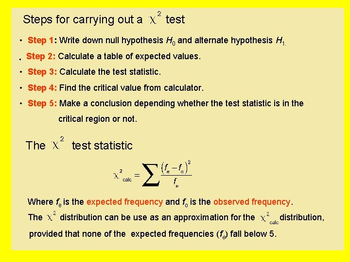
Steps for carrying out a test • Step 1: Write down null hypothesis H 0 and alternate hypothesis H 1. • Step 2: Calculate a table of expected values. • Step 3: Calculate the test statistic. • Step 4: Find the critical value from calculator. • Step 5: Make a conclusion depending whether the test statistic is in the critical region or not. The test statistic Where fe is the expected frequency and fo is the observed frequency. The distribution can be use as an approximation for the provided that none of the expected frequencies (fe) fall below 5. distribution,

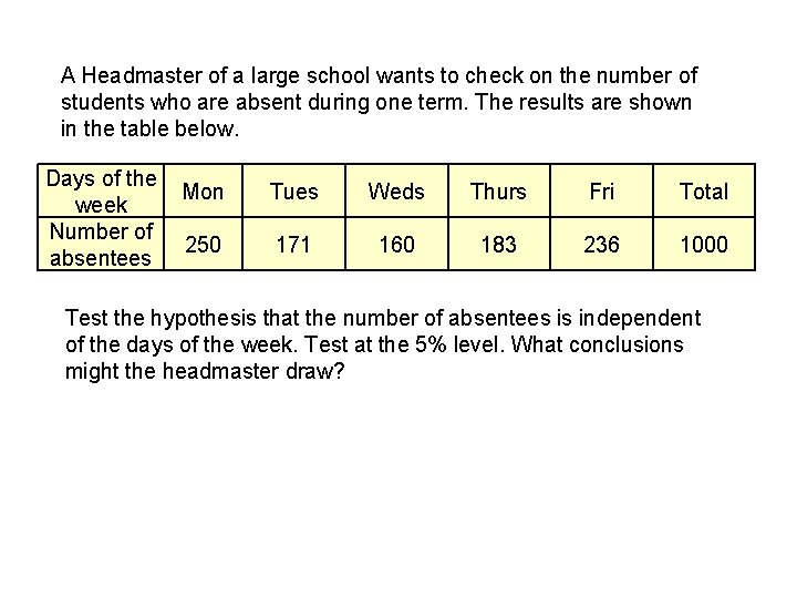
A Headmaster of a large school wants to check on the number of students who are absent during one term. The results are shown in the table below. Days of the week Number of absentees Mon Tues Weds Thurs Fri Total 250 171 160 183 236 1000 Test the hypothesis that the number of absentees is independent of the days of the week. Test at the 5% level. What conclusions might the headmaster draw?

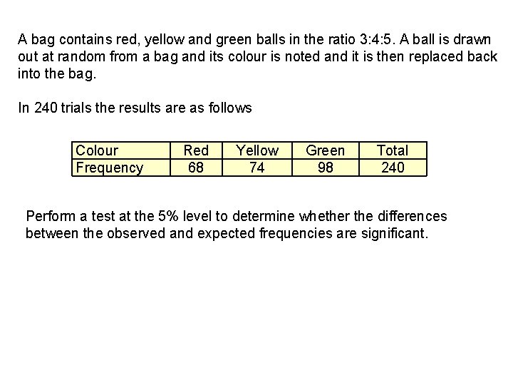
A bag contains red, yellow and green balls in the ratio 3: 4: 5. A ball is drawn out at random from a bag and its colour is noted and it is then replaced back into the bag. In 240 trials the results are as follows Colour Frequency Red 68 Yellow 74 Green 98 Total 240 Perform a test at the 5% level to determine whether the differences between the observed and expected frequencies are significant.

The table below shows the result of planting seeds in rows of 6 and the number of seeds that germinate in each row after a two-week period. Test at the 10% level whether the data can be modelled by a binomial distribution. Number of seeds that germinate (x) Frequency (f) 0 15 1 26 2 21 3 14 4 10 5 9 6 5

The number of telephone calls received by an operator at a hotel between the hours of 9. 00 a. m. and 10. 00 p. m. over a 100 day period is shown in the table below. Number of phone calls Number of days 0 25 1 36 2 16 3 11 4 8 5 4 Determine whether a Poisson distribution with mean 2 can model the above distribution. Test at the 10% level.

A survey is carried out at a supermarket till. When the till opens, the number of customers up to and including the first person to use one of the carrier bags provided by supermarket is recorded. This is repeated on 100 consecutive days. The data is summarised in the table below. Number of customers Frequency (f) 1 79 2 15 3 3 4 3 >4 0 It is thought that this distribution may be modelled by a geometric distribution with parameter p, where p is the probability that a person uses a supermarket carrier bag. a. Calculate the mean and hence obtain an estimate of p. b. Carry out a test at the 5% significance level of goodness of fit of the model to the data.

The heights measured in cm, of a group of students are given in the table below. Determine whether the data can be modelled by a normal distribution. Test at the 5% level. Height in cm 146 -150 151 -155 156 -160 161 -165 166 -170 171 -175 Frequency 10 17 20 14 10 9

Chi-Squared Test for independence on contingency tables Example A driving school examined the results of 100 candidates who were taking their driving test for the first time. They found that of the 40 men, 28 passed and out of the 60 women, 34 passed. Do these results indicate, at the 5% significance, a relationship between the sex of the candidate and the ability to pass first time? Solution The results can be shown in a table, known as a contingency table (read ‘ 2 by 2’) Observed data: Results of first-time candidates Sex Pass Fail Totals Male 28 12 40 Female 34 26 60 Totals 62 38 100

H 0: There is no relationship between the sex of the candidate and the ability to pass first time; the attributes are independent. H 1: There is a relationship between the sex of the candidate and the ability to pass first time; the attributes are not independent. To calculate the expected frequencies: Under H 0 events are independent. Therefore row total grand total column total

We could work through this procedure to give the other expected frequencies, but this is unnecessary, as the other frequencies can be found by using the fact that the sub-totals and totals must agree with those in the observed data: Expected frequencies: Results of first-time candidates Sex Pass Fail Totals Male 24. 8 15. 2 40 Female 37. 2 22. 8 60 62 38 100 Totals Degrees of freedom (v): the number of independent variables (once one expected frequency is known, the others are determined by agreement of totals).

From the tables We test at 5% and reject H 0 if Reject H 0 Therefore fo fe 28 24. 8 0. 4129 12 15. 2 0. 6737 34 37. 2 0. 2753 26 22. 8 0. 4491 1. 8110 As we do not reject H 0 and conclude that these results do not indicate a relationship between the sex of the candidate and the ability to pass first time. Or p-value > 0. 05.

Contingency tables (h rows and k columns) Example In the principality of Viewmania a survey of 200 families known to be regular television viewers was undertaken. They were asked which of the three television channels they watched most during an average week. A summary of their replies is given in the following table, together with the region in which they lived. Region Channel watched most North East South West CCB 1 29 16 42 23 CCB 2 6 11 26 7 VIT 15 3 12 10 Find the expected frequencies on the hypothesis that there is no association between the channel watched most and the region. Use the distribution and a 5% level of significance to test the above hypothesis.

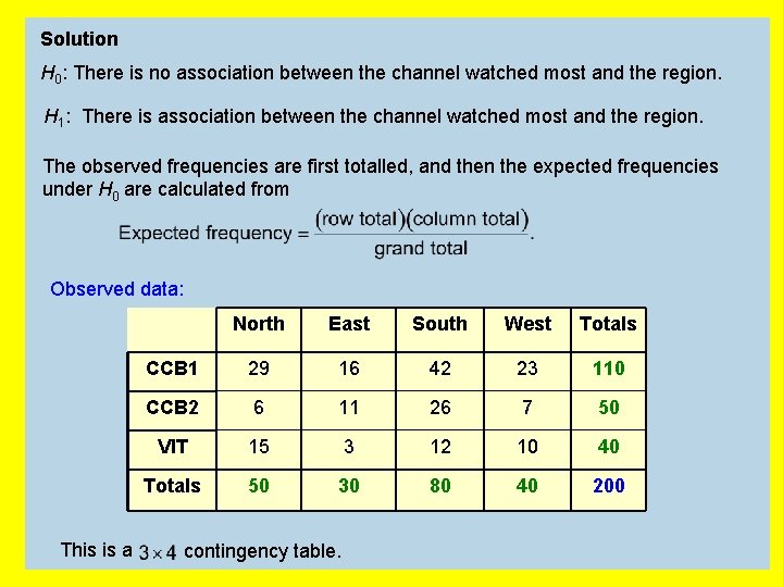
Solution H 0: There is no association between the channel watched most and the region. H 1: There is association between the channel watched most and the region. The observed frequencies are first totalled, and then the expected frequencies under H 0 are calculated from Observed data: This is a North East South West Totals CCB 1 29 16 42 23 110 CCB 2 6 11 26 7 50 VIT 15 3 12 10 40 Totals 50 30 80 40 200 contingency table.

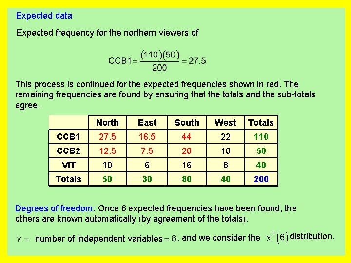
Expected data Expected frequency for the northern viewers of This process is continued for the expected frequencies shown in red. The remaining frequencies are found by ensuring that the totals and the sub-totals agree. North East South West Totals CCB 1 27. 5 16. 5 44 22 110 CCB 2 12. 5 7. 5 20 10 50 VIT 10 6 16 8 40 Totals 50 30 80 40 200 Degrees of freedom: Once 6 expected frequencies have been found, the others are known automatically (by agreement of the totals). number of independent variables , and we consider the distribution.

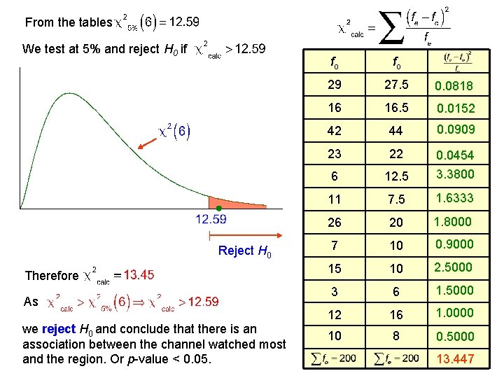
From the tables We test at 5% and reject H 0 if Reject H 0 Therefore As we reject H 0 and conclude that there is an association between the channel watched most and the region. Or p-value < 0. 05. fo fo 29 27. 5 0. 0818 16 16. 5 0. 0152 42 44 0. 0909 23 22 0. 0454 6 12. 5 3. 3800 11 7. 5 1. 6333 26 20 1. 8000 7 10 0. 9000 15 10 2. 5000 3 6 1. 5000 12 16 1. 0000 10 8 0. 5000 13. 447

Example A university sociology department believes that students with a good grade in A-level General Studies tend to do well on Sociology degree courses. To check this it collected information on a random sample of 100 students who had just graduated and who had also taken general studies at A-level. The students’ performance in General Studies was divided two categories, those with A or B and ‘others’. Their degree classes were recorded as Class I, Class III and Fail. The data are given in the table below. Class III Fail Totals Grade A or B 11 22 6 1 40 Others 4 28 24 4 60 Total 15 50 30 5 100 H 0: degree class is independent of General studies A-level performance. H 1: degree class is not independent of General studies A-level performance.

Expected data Class III Fail Totals Grade A or B 6 20 12 2 40 Others 9 30 18 3 60 Total 15 50 30 5 100 New Observed and (Expected) data Class III and Fail Totals Grade A or B 11 (6) 22 (20) 7 (14) 40 Others 4 (9) 28 (30) 28 (21) 60 Total 15 50 35 100