Internal Alignment of the SLD Vertex Detectors David

Internal Alignment of the SLD Vertex Detectors David Jackson, Su Dong, Fred Wickens (RAL, SLAC) • • Overview Vertex Detectors at SLD Residuals used Alignment Matrix I Shape corrections Alignment Matrix II Results + History Comments LHC Alignment Meeting CERN 4 th September 2006 1

Health Warning • Work described was done quite a while ago and over a long period (~1992 - 1999+) • I was never familiar with all of the details, and many of those I did know I have forgotten • It involves a lot of algebra which I will not attempt to duplicate here • I will attempt to answer questions, but may need to pass them on to my co-authors • For the full details see: – D. J. Jackson, D. Su, F. J. Wickens; NIM A 510, 233 (2003) – Or in a slightly expanded form at • http: //www-sldnt. slac. stanford. edu/sldbb/SLDNotes/sld-note 271. pdf • This talk is based heavily on a talk by David Jackson given in early 2005 who I am sure got it right - I take responsibility for any errors introduced here 2

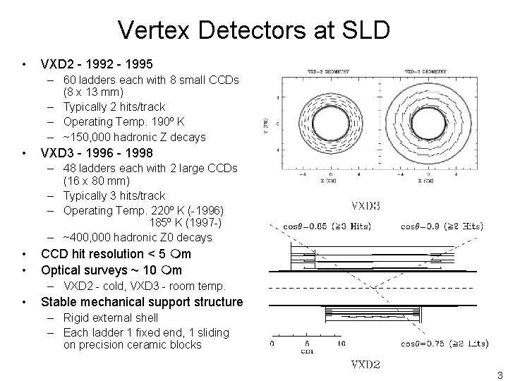
Vertex Detectors at SLD • VXD 2 - 1995 – 60 ladders each with 8 small CCDs (8 x 13 mm) – Typically 2 hits/track – Operating Temp. 190º K – ~150, 000 hadronic Z decays • VXD 3 - 1996 - 1998 – 48 ladders each with 2 large CCDs (16 x 80 mm) – Typically 3 hits/track – Operating Temp. 220º K (-1996) 185º K (1997 -) – ~400, 000 hadronic Z 0 decays • • CCD hit resolution < 5 m Optical surveys ~ 10 m – VXD 2 - cold, VXD 3 - room temp. • Stable mechanical support structure – Rigid external shell – Each ladder 1 fixed end, 1 sliding on precision ceramic blocks 3

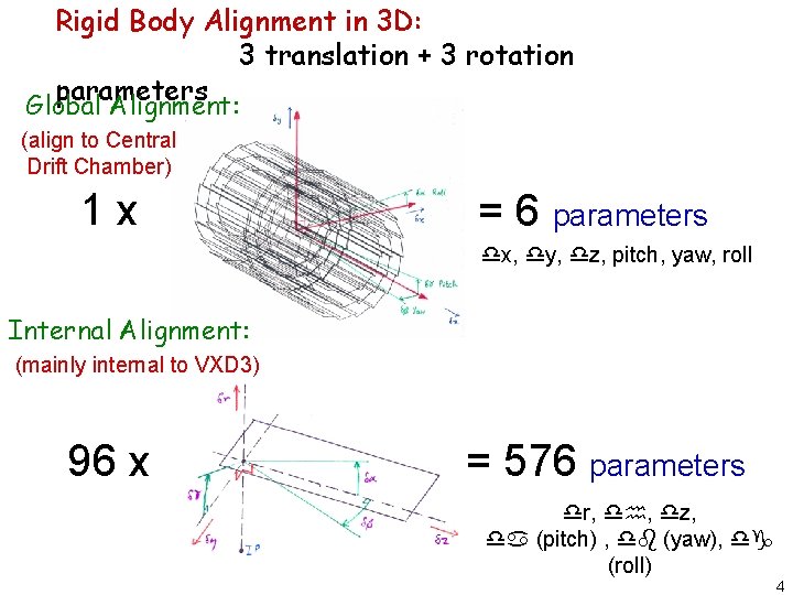
Rigid Body Alignment in 3 D: , 3 translation + 3 rotation parameters Global Alignment: (align to Central Drift Chamber) 1 x = 6 parameters x, y, z, pitch, yaw, roll Internal Alignment: (mainly internal to VXD 3) 96 x = 576 parameters r, , z, (pitch) , (yaw), (roll) 4

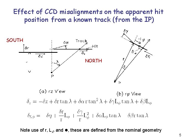
Effect of CCD misalignments on the apparent hit position from a known track (from the IP) SOUTH NORTH Note use of r, L and , these are defined from the nominal geometry 5

General form for Residuals • The CCDs themselves provide the most precise measurements of the track trajectory • Principal idea was to fix a track to two CCD hits and measure a ‘residual’ to a third CCD • The 3 CCDs in each residual contribute to the residual in proportion to a lever-arm weight determined by their relative spacing • e. g. Where the sum is over the 3 CCDs used 6

Residuals types used • ‘doublets’ DOUBLETS – use the small overlap region between the 2 CCDs on a ladder – connect the North/South halves – weight for 3 rd CCD is very small • ‘shingles’ – use the overlap between adjacent CCDs in the same layer – connect the CCDs within each layer – weight for 3 rd CCD is very small • ‘triplets’ – use CCDs from different layers – connect the three layers of the detector SHINGLES TRIPLETS 7

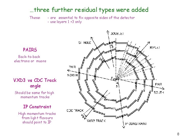
…three further residual types were added These: - are essential to fix opposite sides of the detector - use layers 1 +3 only PAIRS Back-to-back electrons or muons VXD 3 vs CDC Track angle Should be same for high momentum tracks IP Constraint High momentum tracks from light flavours should point to IP 8

Functional forms of residual distributions (treating each CCD as a rigid body) A total of 700 polynomial fits (with 2108 coefficients) 9

Residual fits • For each type of residual n-tuples were accumulated for each unique combination of CCDs • These were then fit to the appropriate functional forms with an automated procedure using MINUIT • E. g. The two fits to one shingle region • This shingle conforms very well to the predicted functional forms • Vertical scatter is due to the intrinsic spatial hit resolution of the CCDs • The procedure included automatic removal of outliers 10

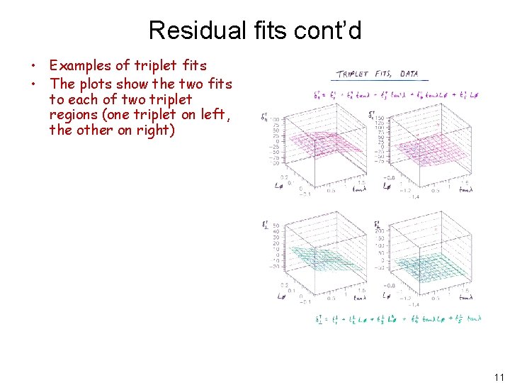
Residual fits cont’d • Examples of triplet fits • The plots show the two fits to each of two triplet regions (one triplet on left, the other on right) 11

Internal Alignment Matrix Equation I The coefficients obtained from the residual fits can also be expressed in terms of a large number of simultaneous linear equations relating them to the unknown alignment parameters; expressing these as a single matrix equation Weight matrix – determined to an extremely good approximation from the known ideal geometry Coefficients measured in residual fits Alignment corrections to be determined 12

Internal Alignment Matrix Equation I • This matrix equation A x = d can now be solved, and our chosen method - using a Singular Value Decomposition (see further details in backup foils) – Is robust – Handles singularities • identifies any unknown parameters which are not constrained by the data – Provides a ‘least squares’ solution • But note that this does not take into account the error and correlation information from the residual fits 13

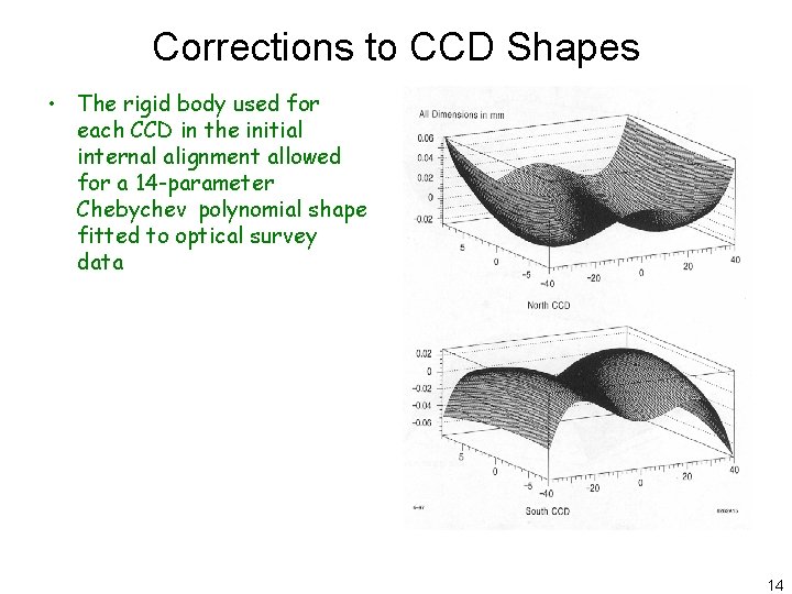
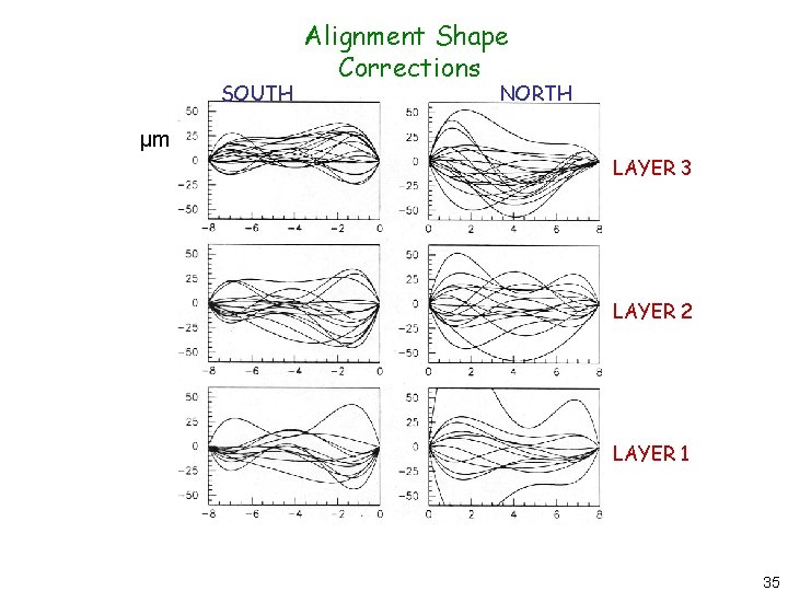
Corrections to CCD Shapes • The rigid body used for each CCD in the initial internal alignment allowed for a 14 -parameter Chebychev polynomial shape fitted to optical survey data 14

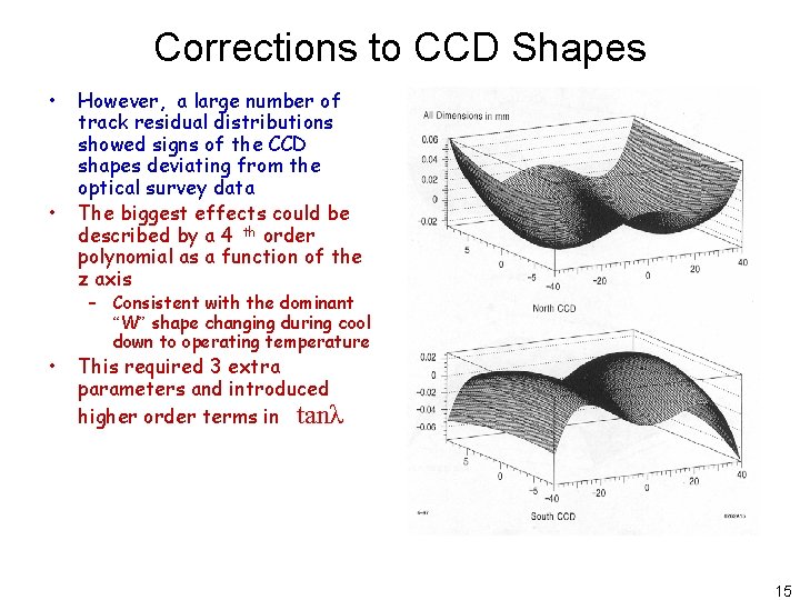
Corrections to CCD Shapes • • • However, a large number of track residual distributions showed signs of the CCD shapes deviating from the optical survey data The biggest effects could be described by a 4 th order polynomial as a function of the z axis – Consistent with the dominant “W” shape changing during cool down to operating temperature This required 3 extra parameters and introduced higher order terms in tanλ 15

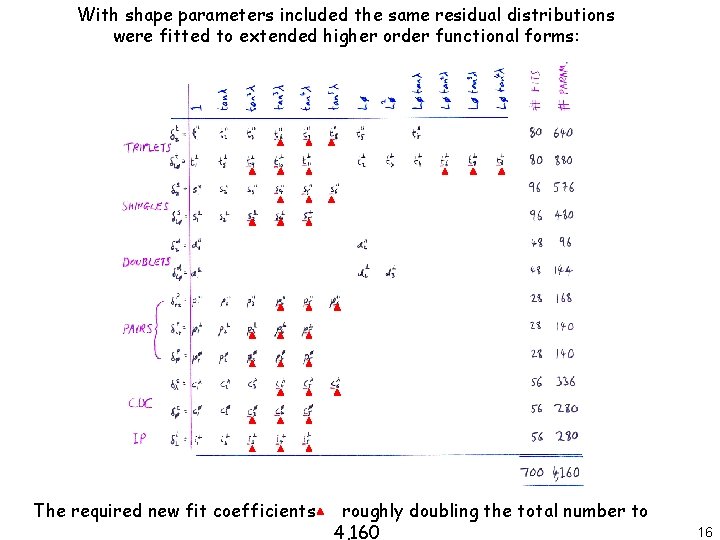
With shape parameters included the same residual distributions were fitted to extended higher order functional forms: The required new fit coefficients roughly doubling the total number to 4, 160 16

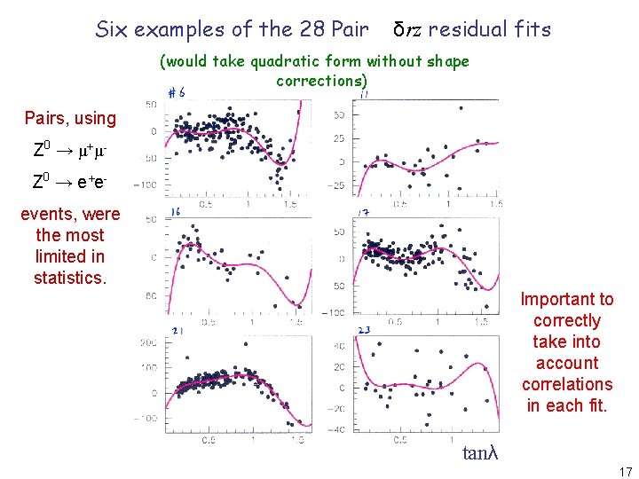
Six examples of the 28 Pair δrz residual fits (would take quadratic form without shape corrections) Pairs, using Z 0 → μ+ μZ 0 → e + eevents, were the most limited in statistics. Important to correctly take into account correlations in each fit. tanλ 17

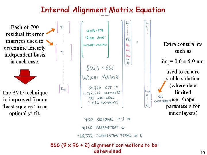
Internal Alignment Matrix Equation II • To remove the correlations and to take account of the errors we redefined the basis of parameters for each residual fit • Thus if each residual fit produces a vector p of n parameters with covariance matrix W • W was decomposed to HHT, where H is a non-singular lower triangular matrix • The parameter vector was transformed to p’ = H-1 p, which has a unit covariance matrix (thus removing correlations and including the quality of each fit) • Gathering together all the elements of the many matrices H-1 from all of the residual fits can produce a single 4160 x 4160 matrix T • Solving the matrix equation TA x = Td = c with SVD now gave a 2 minimization over all the track residuals for the alignment parameters 18

Internal Alignment Matrix Equation II Each of 700 residual fit error matrices used to determine linearly independent basis in each case. δqi = 0. 0 ± 5. 0 μm The SVD technique is improved from a ‘least squares’ to an optimal χ2 fit. used to ensure stable solution (where data limited e. g. shape parameters for inner layers) Extra constraints such as 866 (9 x 96 + 2) alignment corrections to be determined 19

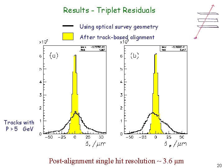
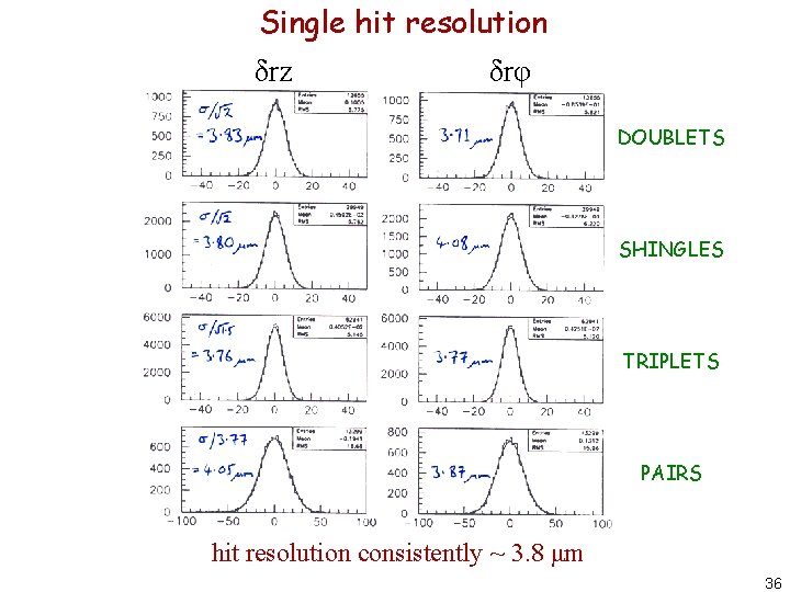
Results - Triplet Residuals Using optical survey geometry After track-based alignment Tracks with P > 5 Ge. V Post-alignment single hit resolution ~ 3. 6 μm 20

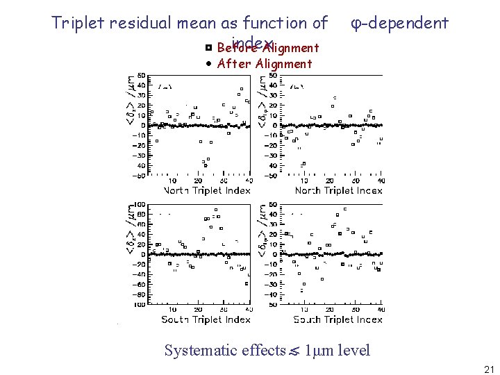
Triplet residual mean as function of index Before Alignment φ-dependent After Alignment Systematic effects ~< 1μm level 21

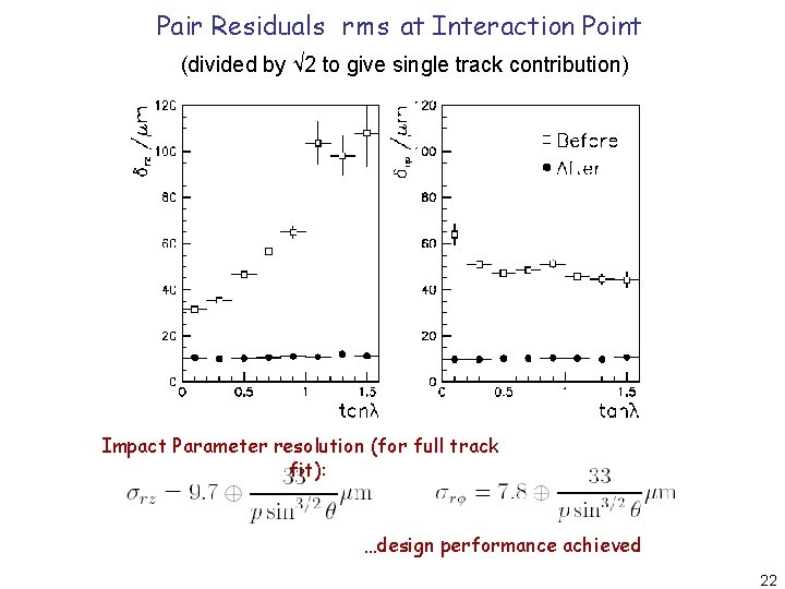
Pair Residuals rms at Interaction Point (divided by √ 2 to give single track contribution) Impact Parameter resolution (for full track fit): …design performance achieved 22

History - VXD 2 • 480 CCDs on 60 ladders • Each ladder treated as a rigid body, apart from a bow – cold optical survey of each ladder during assembly – “hand” corrections for some CCDs based on residual distributions • Residual fits made to doublets and triplets, similar to those described for VXD 3 • Then fitted coefficients to determine 6 degrees of freedom per ladder ( x, y, z, pitch, yaw, bow) – did not include roll as ladders were narrow 23

History - VXD 2 • Initially two separate matrices – Essentially // and perpendicular to length of ladder – Coefficients from residual fits plus constraints – Used SVD technique to solve (and identify underconstrained parameters) • However: – did not take residual fit errors & correlations into account (I. e. “least sq” c. f. Chi-sq) – two dead ladders meant barrel split into two parts • Later used back-to-back pairs to join the two parts - in separate Minuit fit • Process was less polished • But obtained ~5. 5 micron hit resolution 24

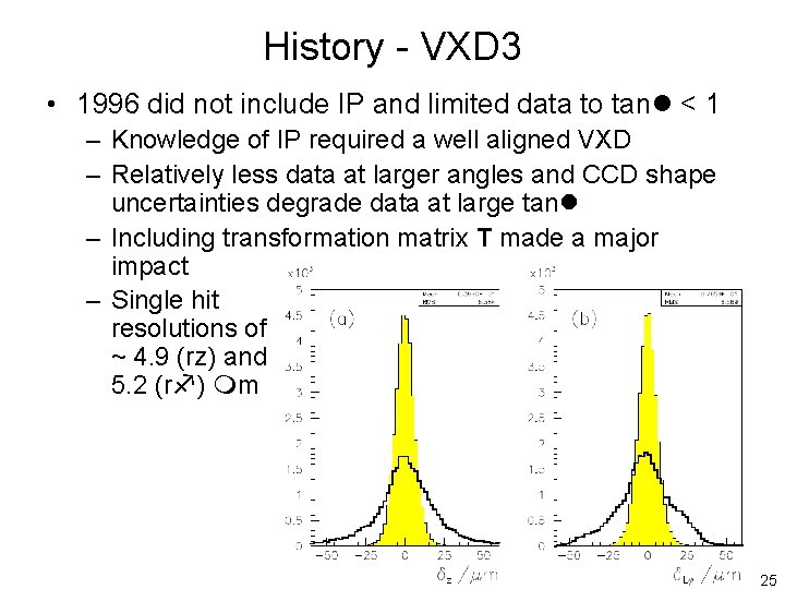
History - VXD 3 • 1996 did not include IP and limited data to tan < 1 – Knowledge of IP required a well aligned VXD – Relatively less data at larger angles and CCD shape uncertainties degrade data at large tan – Including transformation matrix T made a major impact – Single hit resolutions of ~ 4. 9 (rz) and 5. 2 (r ) m 25

History - VXD 3 • 1997 initial fit followed same procedure as 1996 – Single hit resolutions of ~ 4. 9 and 4. 6 m (r improved since 1996 due to removal of some electronic smearing in the detector) • Used this to find average IP over each 30 events, then refitted geometry including IP • 1998 added the shape corrections and extended fits to include data over all tan 26

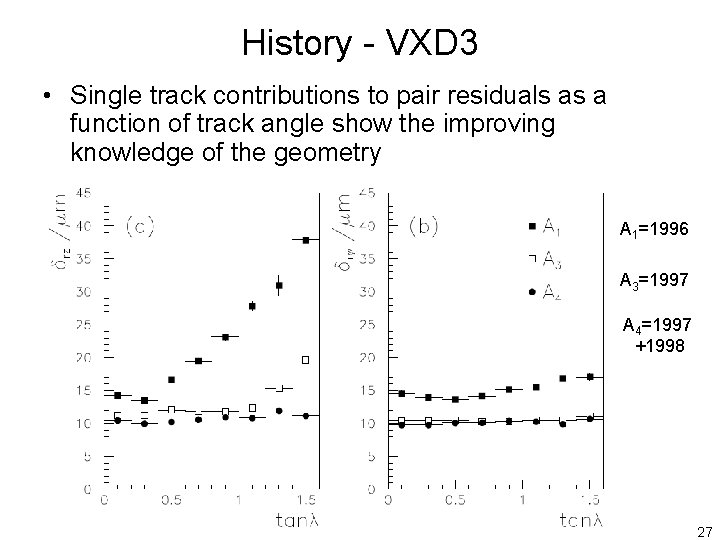
History - VXD 3 • Single track contributions to pair residuals as a function of track angle show the improving knowledge of the geometry A 1=1996 A 3=1997 A 4=1997 +1998 27

History - VXD 3 • Procedure was checked – With Monte-Carlo studies – With 2 nd iteration (made negligible difference) • Examination of residual distributions was important to check for deviations from the assumed functional forms • To understand details of the problem it was found useful to vary the constraints applied to limit the variations of the corrections (e. g. δqi = 0. 0 ± 5. 0 μm ) – But this tuning was not significant to the final results • Some small effects remained in the final residual distributions (e. g. due to slight bow across some doublets) - but were considered too minor to extend the algorithm further 28

Comments for other trackers I The technique - could be used for any system where the required solution takes the form of a perturbation described by O(1000) parameters which are small compared to the dimensions of the system and for which constraining data exists that can be expressed in terms of a set of simultaneous equations for the parameters. Practicalities - we have demonstrated that it was possible (in 1999) to handle simply and reliably the matrices required for the VXD 3 alignment (inversion of sparse matrices of order of 5000 × 1000 elements) using double precision arithmetic in modest times on a standard workstation. Only ∼ 1% or ∼ 35, 000 elements of the final 5026 × 866 design matrix A were given non-zero values 29

Comments for other trackers II Singular Value Decomposition – this alignment technique allowed a robust unbiased solution for SLD; but the method is somewhat secondary in that any technique will have similar statistical dependence on the data and geometry. Alignment is aided by: Symmetry of the detector – greatly assists book-keeping and allows comparison of different parts of the detector. Overlap regions – allows devices to be stitched together with favourable lever arm (data α area of overlap). Large devices – obviously better to have a single element than two with an overlap. 30

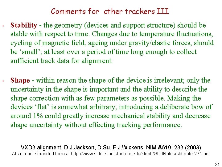
Comments for other trackers III • Stability - the geometry (devices and support structure) should be stable with respect to time. Changes due to temperature fluctuations, cycling of magnetic field, ageing under gravity/elastic forces, should be ‘small’; at least over a period of time long enough to collect sufficient track data for alignment. • Shape - within reason the shape of the device is irrelevant; only the uncertainty in the shape is important and the ability to describe the shape correction with as few parameters as possible. Making the devices ‘flat’ is somewhat arbitrary; introducing a deliberate bow of around 1% could greatly increase mechanical stability and decrease shape uncertainty without effecting tracking performance. VXD 3 alignment: D. J. Jackson, D. Su, F. J. Wickens; NIM A 510, 233 (2003) Also in an expanded form at http: //www-sldnt. slac. stanford. edu/sldbb/SLDNotes/sld-note-271. pdf 31

Back-up slides 32

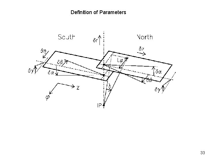
Definition of Parameters 33

CCD Shape Corrections An arbitrary surface shape can be introduced by setting: δr → δr + f (z) For convenience the base of the CCDs (each 8 cm in length) was taken as: z. B = (r tanλ)/8 34

SOUTH Alignment Shape Corrections NORTH μm LAYER 3 LAYER 2 LAYER 1 35

Single hit resolution δrz δrφ DOUBLETS SHINGLES TRIPLETS PAIRS hit resolution consistently ~ 3. 8 μm 36

SOUTH NORTH 37

Singular Value Decomposition mxm othogonal mxn diag. nxn orthogonal s 1…sr are called the ‘singular values’ of matrix A; si ~ 0 corresponds to a singularity of A Here’s the SVD trick: define the inverse A+ = VS+UT with S+ = . 1/s 1. 1/s 2. . . 1/sr with 1/si = 0 if si ~ 0 Then if Ax = b (for vectors x, b) The solution x 0 = A+b is such that: | Ax 0 – b | has minimum length That is, the SVD technique gives the closest ‘least squares’ solution for an over-constrained (and possibly singular) system 38