Intermediate Macroeconomics Chapter 6 The Neoclassical ISLM Model

Intermediate Macroeconomics Chapter 6 The Neoclassical IS-LM Model

The Neoclassical IS - LM Model • • • IS-LM Model The IS Curve The LM Curve IS-LM Equilibrium Fiscal and Monetary Policy Intermediate Macroeconomics

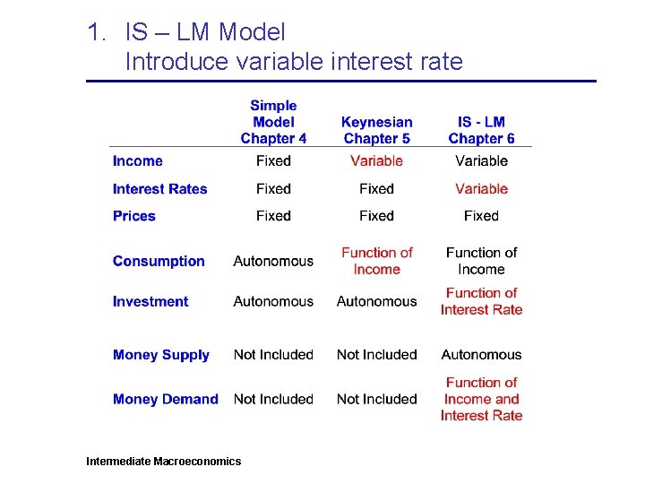
1. IS – LM Model Introduce variable interest rate Intermediate Macroeconomics

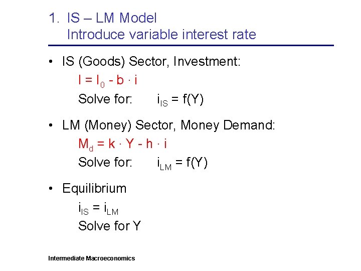
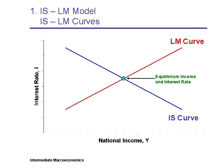
1. IS – LM Model Introduce variable interest rate • IS (Goods) Sector, Investment: I = I 0 - b · i Solve for: i. IS = f(Y) • LM (Money) Sector, Money Demand: Md = k · Y - h · i Solve for: i. LM = f(Y) • Equilibrium i. IS = i. LM Solve for Y Intermediate Macroeconomics

1. IS – LM Model IS – LM Curves LM Curve Equilibrium Income and Interest Rate IS Curve Intermediate Macroeconomics

1. IS – LM Model Fiscal and monetary policy • Fiscal Policy (spending and taxes) – shifts IS curve – increase in spending or cut in taxes shifts IS curve to the right • Monetary Policy (money supply) – shifts LM curve – increase in money supply shifts LM curve to the right Intermediate Macroeconomics

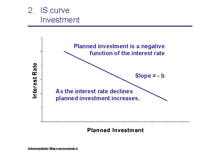
2. IS curve Investment Planned investment is a negative function of the interest rate Slope = - b As the interest rate declines planned investment increases. Intermediate Macroeconomics

2. IS Curve The “goods” market Given: AE = C + I + G + NX C = C 0 + c · YD I = I 0 - b · i G = G 0 NX = NX 0 YD = Y – t · Y + TR 0 Intermediate Macroeconomics

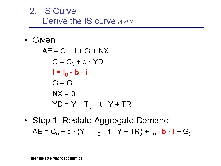
2. IS Curve Derive the IS curve (1 of 3) • Given: AE = C + I + G + NX C = C 0 + c · YD I = I 0 - b · i G = G 0 NX = 0 YD = Y – T 0 – t · Y + TR • Step 1. Restate Aggregate Demand: AE = C 0 + c · (Y – T 0 – t · Y + TR) + I 0 - b · i + G 0 Intermediate Macroeconomics

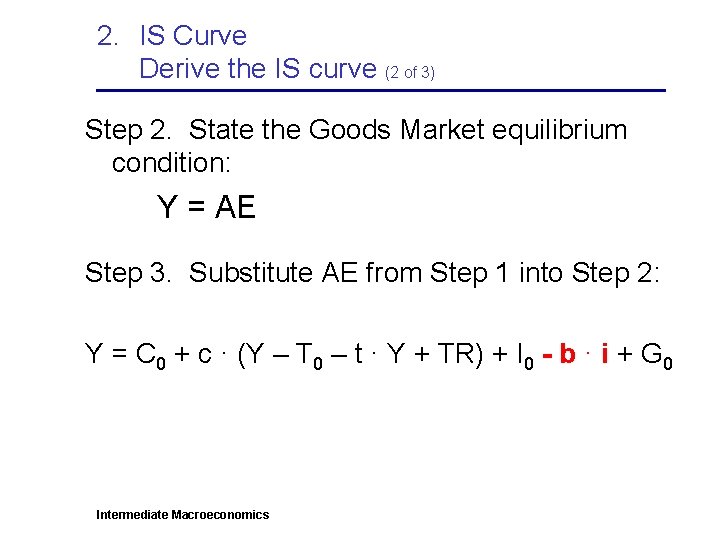
2. IS Curve Derive the IS curve (2 of 3) Step 2. State the Goods Market equilibrium condition: Y = AE Step 3. Substitute AE from Step 1 into Step 2: Y = C 0 + c · (Y – T 0 – t · Y + TR) + I 0 - b · i + G 0 Intermediate Macroeconomics

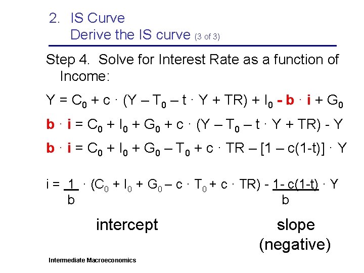
2. IS Curve Derive the IS curve (3 of 3) Step 4. Solve for Interest Rate as a function of Income: Y = C 0 + c · (Y – T 0 – t · Y + TR) + I 0 - b · i + G 0 b · i = C 0 + I 0 + G 0 + c · (Y – T 0 – t · Y + TR) - Y b · i = C 0 + I 0 + G 0 – T 0 + c · TR – [1 – c(1 -t)] · Y i = 1 · (C 0 + I 0 + G 0 – c · T 0 + c · TR) - 1 - c(1 -t) · Y b b intercept Intermediate Macroeconomics slope (negative)

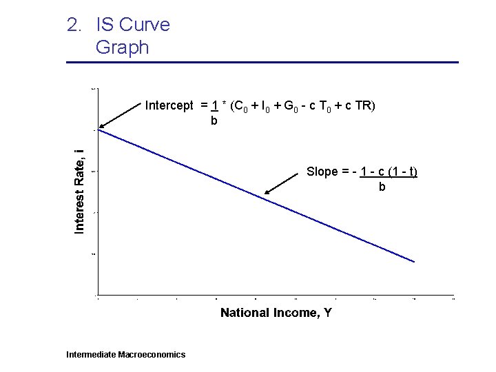
2. IS Curve Graph Intercept = 1 * (C 0 + I 0 + G 0 - c T 0 + c TR) b Slope = - 1 - c (1 - t) b Intermediate Macroeconomics

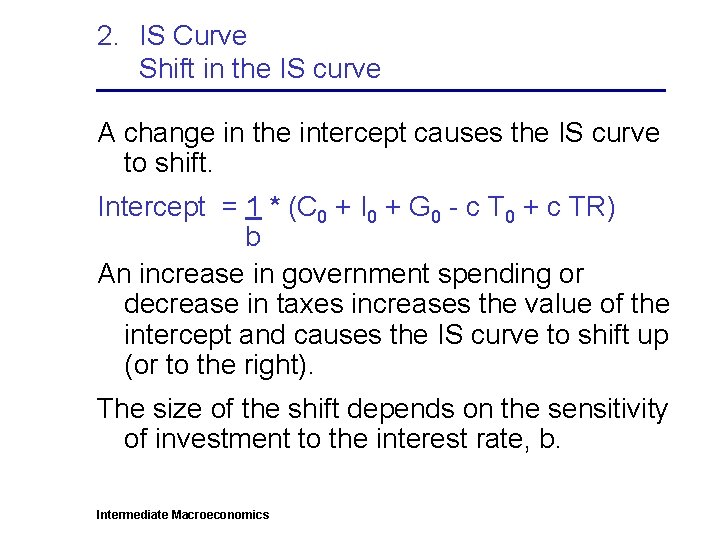
2. IS Curve Shift in the IS curve A change in the intercept causes the IS curve to shift. Intercept = 1 * (C 0 + I 0 + G 0 - c T 0 + c TR) b An increase in government spending or decrease in taxes increases the value of the intercept and causes the IS curve to shift up (or to the right). The size of the shift depends on the sensitivity of investment to the interest rate, b. Intermediate Macroeconomics

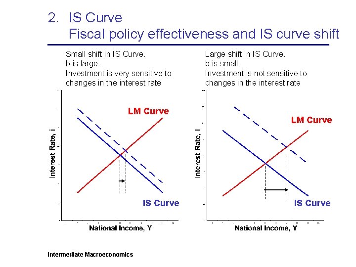
2. IS Curve Fiscal policy effectiveness and IS curve shift Small shift in IS Curve. b is large. Investment is very sensitive to changes in the interest rate LM Curve IS Curve Intermediate Macroeconomics Large shift in IS Curve. b is small. Investment is not sensitive to changes in the interest rate LM Curve IS Curve

2. IS Curve Fiscal policy effectiveness and IS curve shift • Small shift in IS curve – Classical view, fiscal policy ineffective – Increase in government spending raises interest rate, which crowds out (reduces) investment spending. Net increase in aggregate spending may be small • Large shift in IS curve – Keynesian view, fiscal policy effective. – Increase in government spending may raise the interest rate but has no effect on investment. Get big bang for buck. Intermediate Macroeconomics

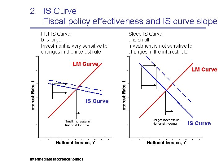
2. IS Curve Slope of the curve Effectiveness of fiscal policy also depends on the slope of the IS curve Slope = - 1 - c (1 - t) b Keynesian: small b, steep curve fiscal policy more effective Classical: large b, flat curve fiscal policy less effective Intermediate Macroeconomics

2. IS Curve Fiscal policy effectiveness and IS curve slope Flat IS Curve. b is large. Investment is very sensitive to changes in the interest rate Steep IS Curve. b is small. Investment is not sensitive to changes in the interest rate LM Curve IS Curve Small increase in National Income Intermediate Macroeconomics Larger increase in National Income IS Curve

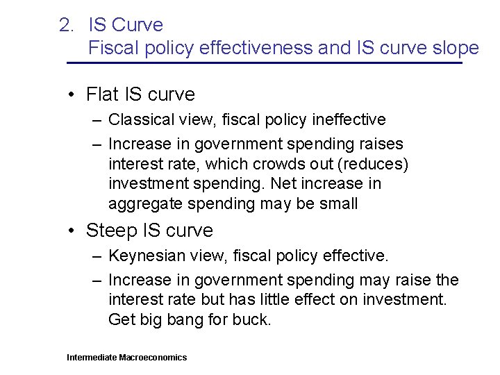
2. IS Curve Fiscal policy effectiveness and IS curve slope • Flat IS curve – Classical view, fiscal policy ineffective – Increase in government spending raises interest rate, which crowds out (reduces) investment spending. Net increase in aggregate spending may be small • Steep IS curve – Keynesian view, fiscal policy effective. – Increase in government spending may raise the interest rate but has little effect on investment. Get big bang for buck. Intermediate Macroeconomics

3. LM Curve Money Supply and Money Demand • Money Supply: – assumed to be a some fixed level • Money Demand: – negative function of interest rate. People hold more money when interest rates decline. – positive function of income. People hold more money as their income increases. Intermediate Macroeconomics

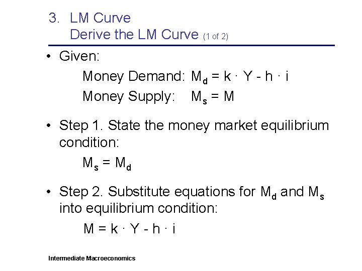
3. LM Curve Derive the LM Curve (1 of 2) • Given: Money Demand: Md = k · Y - h · i Money Supply: Ms = M • Step 1. State the money market equilibrium condition: Ms = Md • Step 2. Substitute equations for Md and Ms into equilibrium condition: M=k·Y-h·i Intermediate Macroeconomics

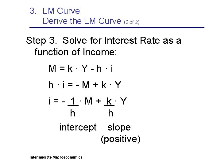
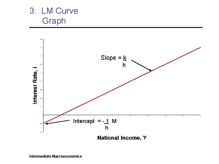
3. LM Curve Derive the LM Curve (2 of 2) Step 3. Solve for Interest Rate as a function of Income: M=k·Y-h·i h·i=-M+k·Y i=- 1·M+ k·Y h h intercept slope (positive) Intermediate Macroeconomics

3. LM Curve Graph Slope = k h Intercept = - 1 M h Intermediate Macroeconomics

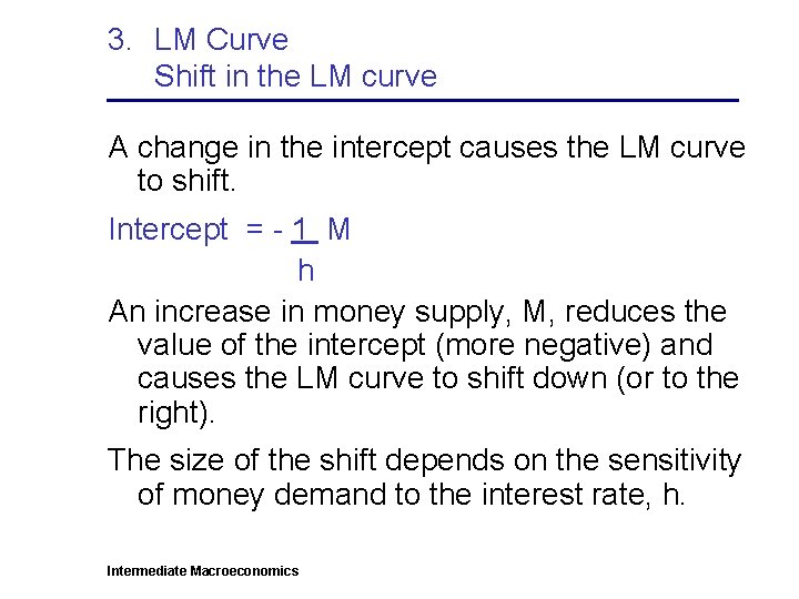
3. LM Curve Shift in the LM curve A change in the intercept causes the LM curve to shift. Intercept = - 1 M h An increase in money supply, M, reduces the value of the intercept (more negative) and causes the LM curve to shift down (or to the right). The size of the shift depends on the sensitivity of money demand to the interest rate, h. Intermediate Macroeconomics

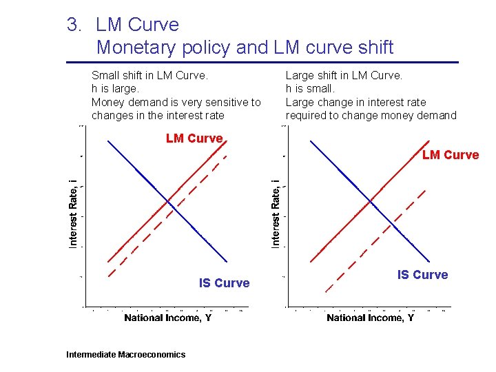
3. LM Curve Monetary policy and LM curve shift Small shift in LM Curve. h is large. Money demand is very sensitive to changes in the interest rate Large shift in LM Curve. h is small. Large change in interest rate required to change money demand LM Curve IS Curve Intermediate Macroeconomics IS Curve

3. LM Curve Monetary policy and LM curve shift • Small shift in LM curve – Keynesian view, monetary policy ineffective – Increase in money supply is met by an increase in money demand without a significant decline in the interest rate. No stimulus to investment spending. • Large shift in LM curve – Classical view, monetary policy effective. – Increase in money supply leads to a large decline in the interest rate in order to increase money demand. Increases investment spending. Intermediate Macroeconomics

3. LM Curve Slope of the LM curve Effectiveness of monetary policy also depends on the slope of the LM curve Slope = k h Keynesian: large h, flat curve monetary policy less effective Classical: small h, steep curve monetary policy more effective Note: little debate over change in money demand with change in income, k. Intermediate Macroeconomics

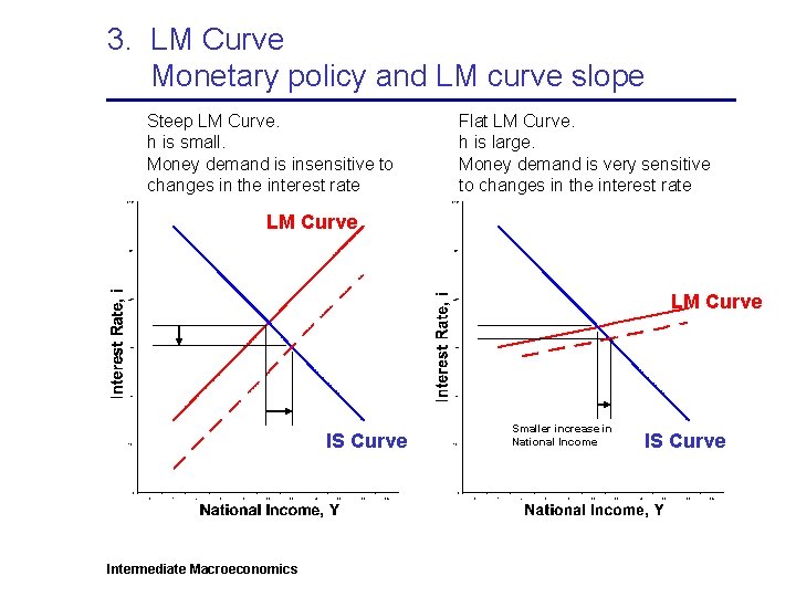
3. LM Curve Monetary policy and LM curve slope Steep LM Curve. h is small. Money demand is insensitive to changes in the interest rate Flat LM Curve. h is large. Money demand is very sensitive to changes in the interest rate LM Curve IS Curve Intermediate Macroeconomics Smaller increase in National Income IS Curve

3. LM Curve Monetary policy and LM curve slope • Flat LM curve – Keynesian view, monetary policy ineffective – Increase in money supply has little or no effect on the interest rate. Money demand adjusts to match money supply. No change in interest rate means no change in investment and aggregate spending • Steep LM curve – Classical view, monetary policy effective. – Increase in money supply lowers the interest rate, which increases investment spending. Intermediate Macroeconomics

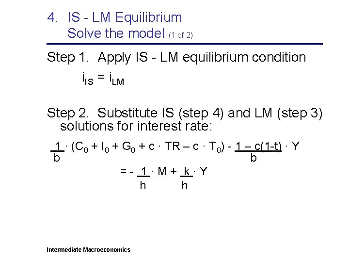
4. IS - LM Equilibrium Solve the model (1 of 2) Step 1. Apply IS - LM equilibrium condition i. IS = i. LM Step 2. Substitute IS (step 4) and LM (step 3) solutions for interest rate: 1 · (C 0 + I 0 + G 0 + c · TR – c · T 0) - 1 – c(1 -t) · Y b b =- 1·M+ k·Y h h Intermediate Macroeconomics

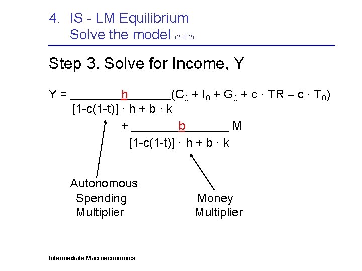
4. IS - LM Equilibrium Solve the model (2 of 2) Step 3. Solve for Income, Y Y= h (C 0 + I 0 + G 0 + c · TR – c · T 0) [1 -c(1 -t)] · h + b · k + b M [1 -c(1 -t)] · h + b · k Autonomous Spending Multiplier Intermediate Macroeconomics Money Multiplier

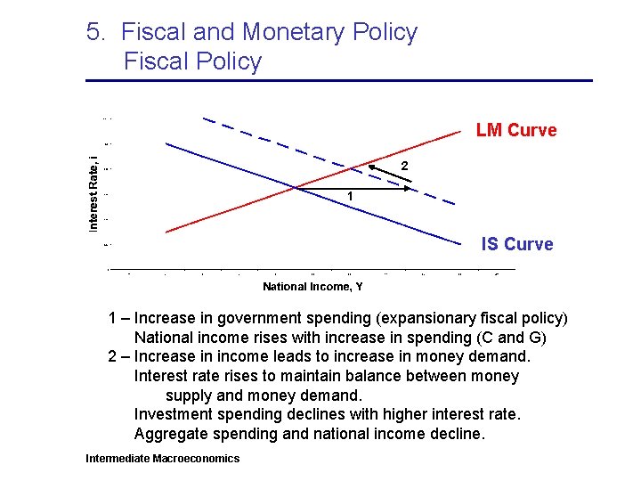
5. Fiscal and Monetary Policy Fiscal Policy LM Curve 2 1 IS Curve 1 – Increase in government spending (expansionary fiscal policy) National income rises with increase in spending (C and G) 2 – Increase in income leads to increase in money demand. Interest rate rises to maintain balance between money supply and money demand. Investment spending declines with higher interest rate. Aggregate spending and national income decline. Intermediate Macroeconomics

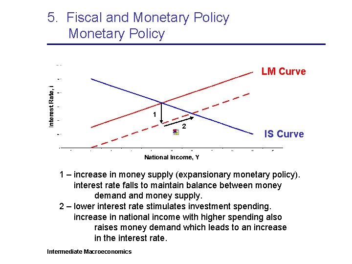
5. Fiscal and Monetary Policy LM Curve 1 2 IS Curve 1 – increase in money supply (expansionary monetary policy). interest rate falls to maintain balance between money demand money supply. 2 – lower interest rate stimulates investment spending. increase in national income with higher spending also raises money demand which leads to an increase in the interest rate. Intermediate Macroeconomics

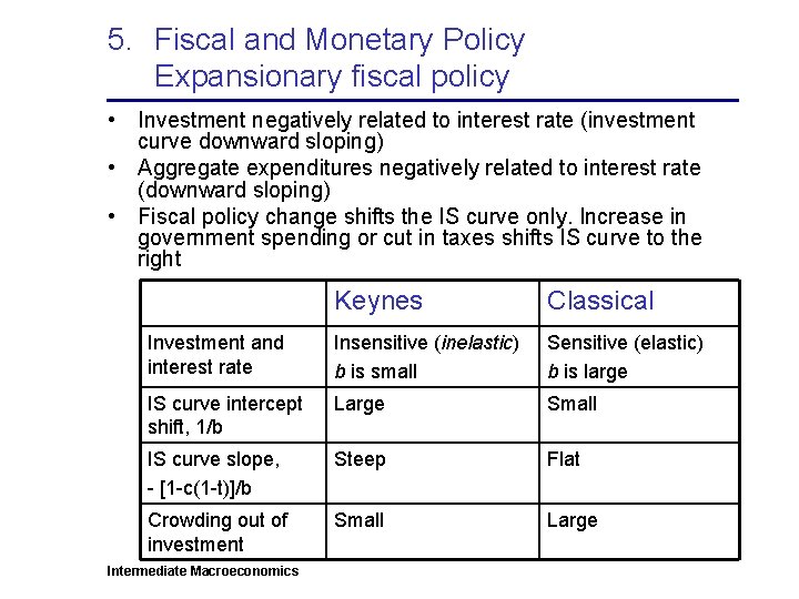
5. Fiscal and Monetary Policy Expansionary fiscal policy • Investment negatively related to interest rate (investment curve downward sloping) • Aggregate expenditures negatively related to interest rate (downward sloping) • Fiscal policy change shifts the IS curve only. Increase in government spending or cut in taxes shifts IS curve to the right Keynes Classical Investment and interest rate Insensitive (inelastic) b is small Sensitive (elastic) b is large IS curve intercept shift, 1/b Large Small IS curve slope, - [1 -c(1 -t)]/b Steep Flat Crowding out of investment Small Large Intermediate Macroeconomics

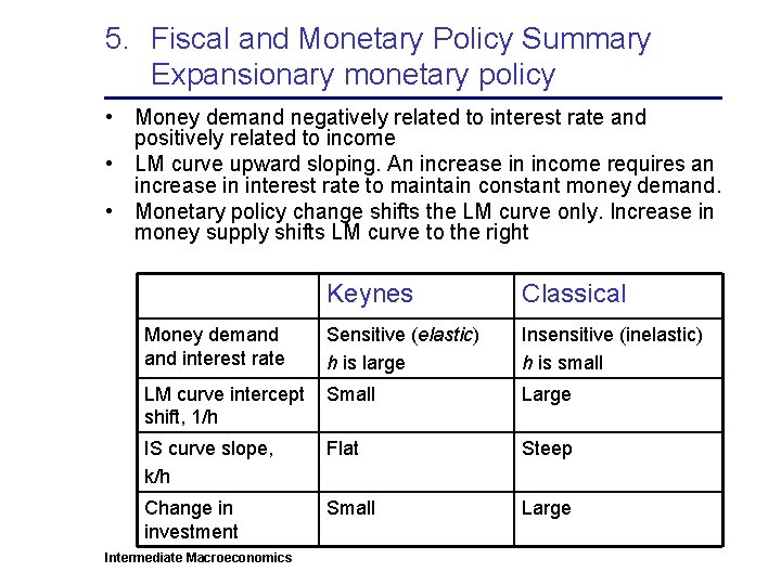
5. Fiscal and Monetary Policy Summary Expansionary monetary policy • Money demand negatively related to interest rate and positively related to income • LM curve upward sloping. An increase in income requires an increase in interest rate to maintain constant money demand. • Monetary policy change shifts the LM curve only. Increase in money supply shifts LM curve to the right Keynes Classical Money demand interest rate Sensitive (elastic) h is large Insensitive (inelastic) h is small LM curve intercept shift, 1/h Small Large IS curve slope, k/h Flat Steep Change in investment Small Large Intermediate Macroeconomics