Intermediate Macroeconomics Chapter 10 Consumption and Savings Consumption

Intermediate Macroeconomics Chapter 10 Consumption and Savings

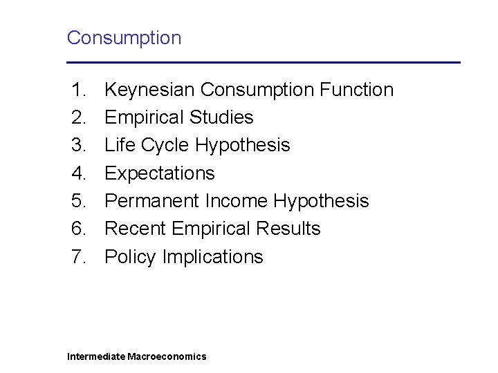
Consumption 1. 2. 3. 4. 5. 6. 7. Keynesian Consumption Function Empirical Studies Life Cycle Hypothesis Expectations Permanent Income Hypothesis Recent Empirical Results Policy Implications Intermediate Macroeconomics

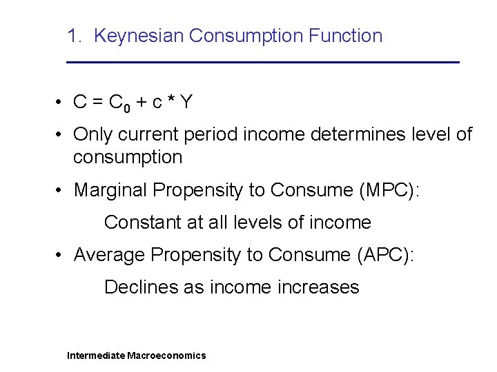
1. Keynesian Consumption Function • C = C 0 + c * Y • Only current period income determines level of consumption • Marginal Propensity to Consume (MPC): Constant at all levels of income • Average Propensity to Consume (APC): Declines as income increases Intermediate Macroeconomics

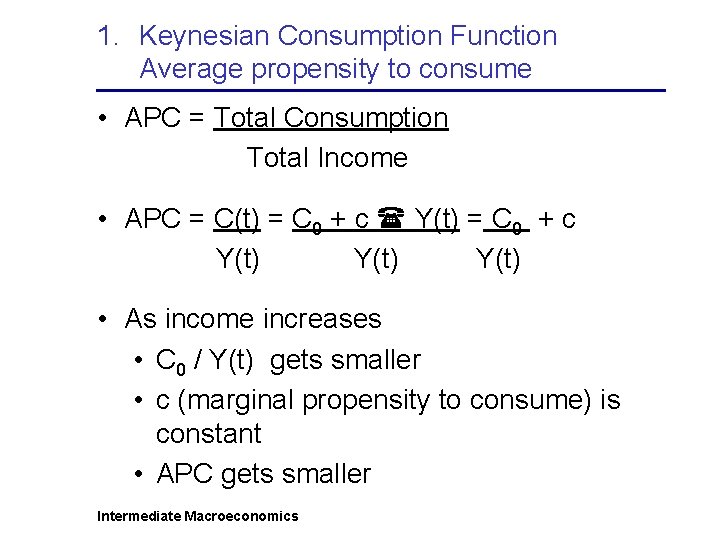
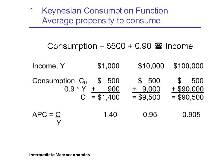
1. Keynesian Consumption Function Average propensity to consume • APC = Total Consumption Total Income • APC = C(t) = C 0 + c Y(t) = C 0 + c Y(t) • As income increases • C 0 / Y(t) gets smaller • c (marginal propensity to consume) is constant • APC gets smaller Intermediate Macroeconomics

1. Keynesian Consumption Function Average propensity to consume Consumption = $500 + 0. 90 Income Intermediate Macroeconomics

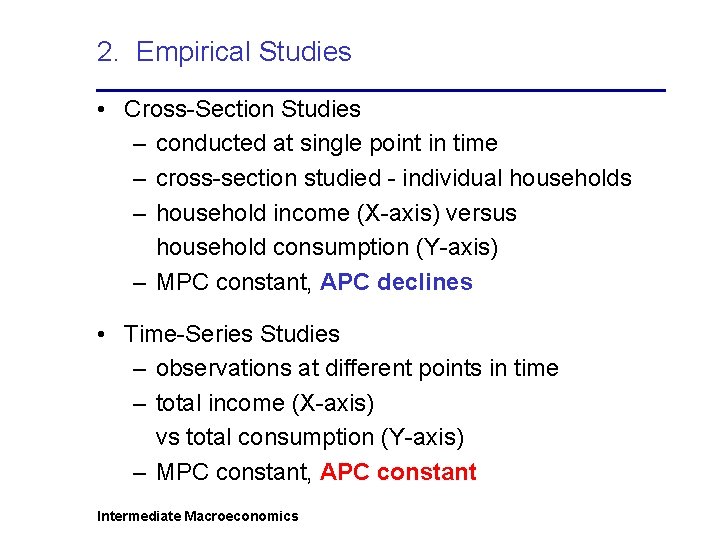
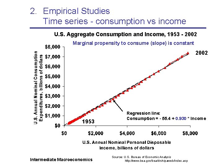
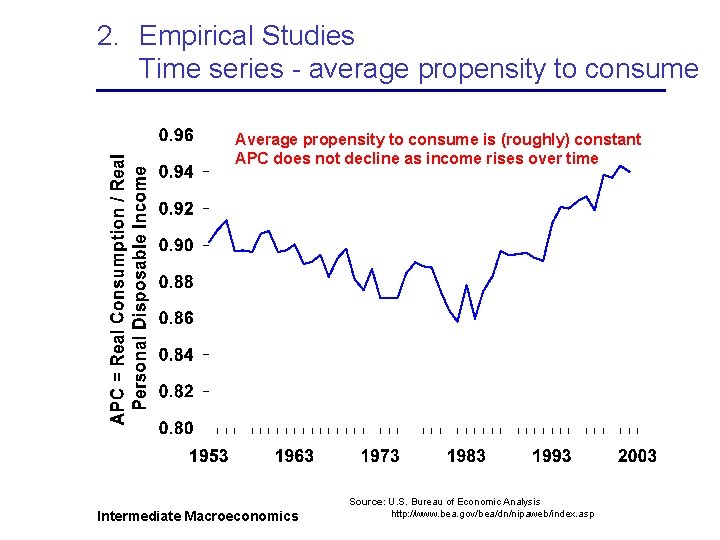
2. Empirical Studies • Cross-Section Studies – conducted at single point in time – cross-section studied - individual households – household income (X-axis) versus household consumption (Y-axis) – MPC constant, APC declines • Time-Series Studies – observations at different points in time – total income (X-axis) vs total consumption (Y-axis) – MPC constant, APC constant Intermediate Macroeconomics

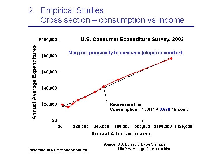
2. Empirical Studies Cross section – consumption vs income U. S. Consumer Expenditure Survey, 2002 Marginal propensity to consume (slope) is constant Intermediate Macroeconomics Source: U. S. Bureau of Labor Statistics http: //www. bls. gov/cex/home. htm

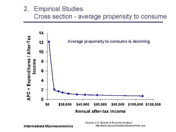
2. Empirical Studies Cross section - average propensity to consume Average propensity to consume is declining Intermediate Macroeconomics Source: U. S. Bureau of Economic Analysis http: //www. bea. gov/bea/dn/nipaweb/index. asp

2. Empirical Studies Time series - consumption vs income U. S. Aggregate Consumption and Income, 1953 - 2002 Marginal propensity to consume (slope) is constant 2002 1953 Intermediate Macroeconomics Regression line: Consumption = - 55. 4 + 0. 930 * Income Source: U. S. Bureau of Economic Analysis http: //www. bea. gov/bea/dn/nipaweb/index. asp

2. Empirical Studies Time series - average propensity to consume Average propensity to consume is (roughly) constant APC does not decline as income rises over time Intermediate Macroeconomics Source: U. S. Bureau of Economic Analysis http: //www. bea. gov/bea/dn/nipaweb/index. asp

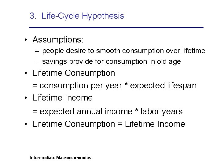
3. Life-Cycle Hypothesis • Assumptions: – people desire to smooth consumption over lifetime – savings provide for consumption in old age • Lifetime Consumption = consumption per year * expected lifespan • Lifetime Income = expected annual income * labor years • Lifetime Consumption = Lifetime Income Intermediate Macroeconomics

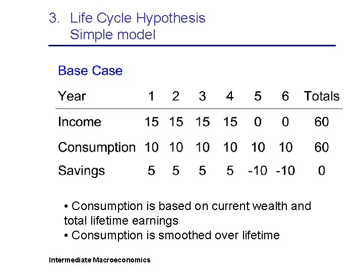
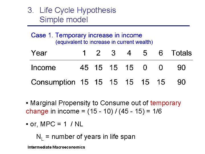
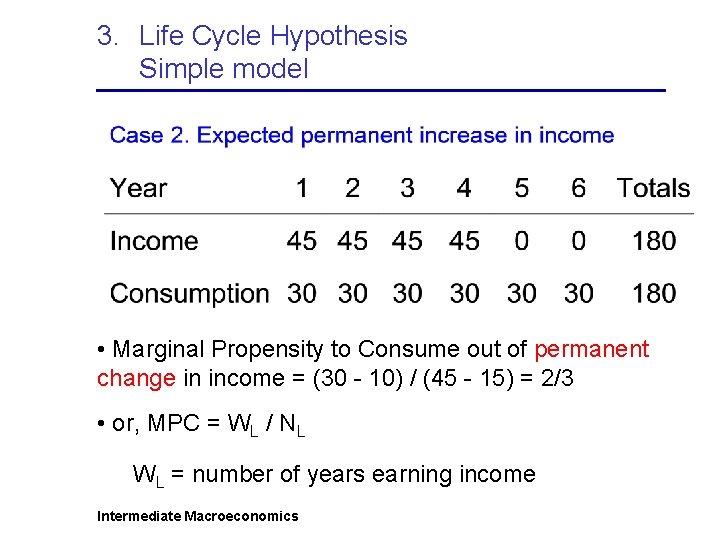
3. Life Cycle Hypothesis Simple model • Consumption is based on current wealth and total lifetime earnings • Consumption is smoothed over lifetime Intermediate Macroeconomics

3. Life Cycle Hypothesis Simple model • Marginal Propensity to Consume out of temporary change in income = (15 - 10) / (45 - 15) = 1/6 • or, MPC = 1 / NL NL = number of years in life span Intermediate Macroeconomics

3. Life Cycle Hypothesis Simple model • Marginal Propensity to Consume out of permanent change in income = (30 - 10) / (45 - 15) = 2/3 • or, MPC = WL / NL WL = number of years earning income Intermediate Macroeconomics

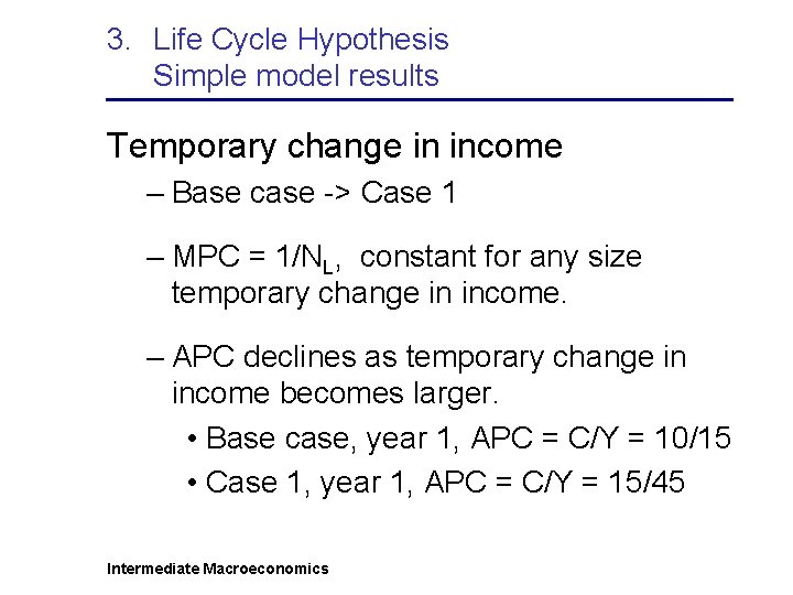
3. Life Cycle Hypothesis Simple model results Temporary change in income – Base case -> Case 1 – MPC = 1/NL, constant for any size temporary change in income. – APC declines as temporary change in income becomes larger. • Base case, year 1, APC = C/Y = 10/15 • Case 1, year 1, APC = C/Y = 15/45 Intermediate Macroeconomics

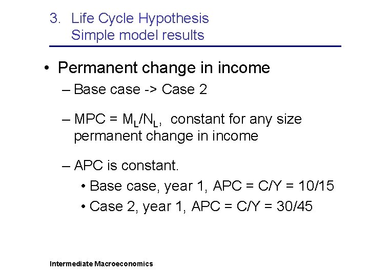
3. Life Cycle Hypothesis Simple model results • Permanent change in income – Base case -> Case 2 – MPC = ML/NL, constant for any size permanent change in income – APC is constant. • Base case, year 1, APC = C/Y = 10/15 • Case 2, year 1, APC = C/Y = 30/45 Intermediate Macroeconomics

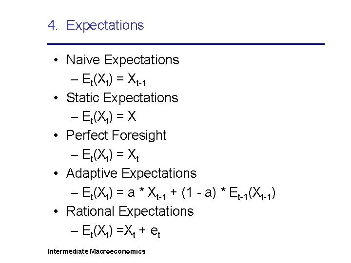
4. Expectations • Naive Expectations – Et(Xt) = Xt-1 • Static Expectations – Et(Xt) = X • Perfect Foresight – Et(Xt) = Xt • Adaptive Expectations – Et(Xt) = a * Xt-1 + (1 - a) * Et-1(Xt-1) • Rational Expectations – Et(Xt) =Xt + et Intermediate Macroeconomics

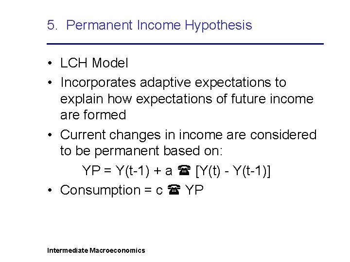
5. Permanent Income Hypothesis • LCH Model • Incorporates adaptive expectations to explain how expectations of future income are formed • Current changes in income are considered to be permanent based on: YP = Y(t-1) + a [Y(t) - Y(t-1)] • Consumption = c YP Intermediate Macroeconomics

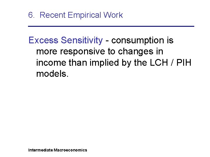
6. Recent Empirical Work Excess Sensitivity - consumption is more responsive to changes in income than implied by the LCH / PIH models. Intermediate Macroeconomics

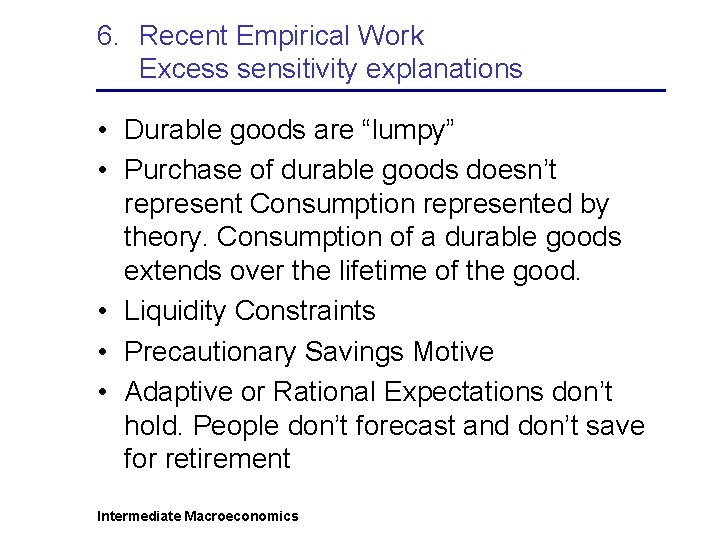
6. Recent Empirical Work Excess sensitivity explanations • Durable goods are “lumpy” • Purchase of durable goods doesn’t represent Consumption represented by theory. Consumption of a durable goods extends over the lifetime of the good. • Liquidity Constraints • Precautionary Savings Motive • Adaptive or Rational Expectations don’t hold. People don’t forecast and don’t save for retirement Intermediate Macroeconomics

7. Policy Implications • Temporary Tax Changes • Ricardian Equivalence • Higher Interest Rates • Social Security Intermediate Macroeconomics