Interferometric FWI for Time Lapse Data By Mrinal

Interferometric FWI for Time. Lapse Data By Mrinal Sinha King Abdullah University of Science and Technology

Outline • Motivation s • Theory of Interferometric FWI • Numerical Examples • Conclusions FWI g IFWI

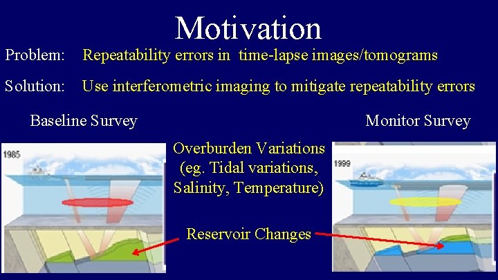
Motivation Problem: Repeatability errors in time-lapse images/tomograms Solution: Use interferometric imaging to mitigate repeatability errors Baseline Survey Monitor Survey Overburden Variations (eg. Tidal variations, Salinity, Temperature) Reservoir Changes

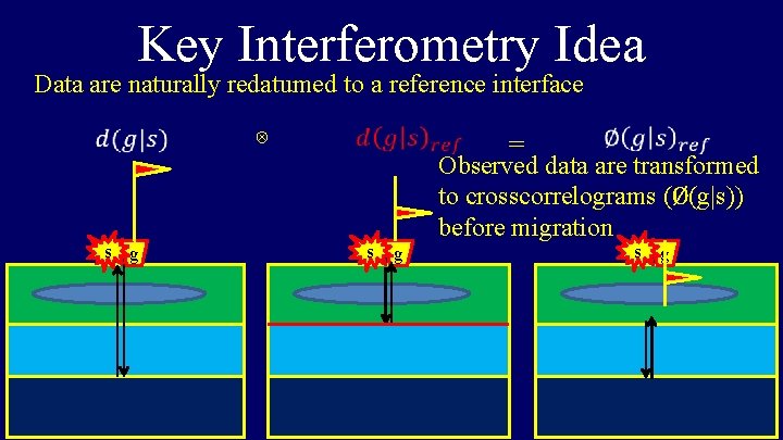
Key Interferometry Idea Data are naturally redatumed to a reference interface ⊗ s g = Observed data are transformed to crosscorrelograms (Ø(g|s)) before migration s g

Motivation Solution: Use interferometric imaging to mitigate repeatability errors Baseline Survey s g Repeatability is improved due to redatuming Monitor Survey s g Reservoir changes decoupled from overburden variations

Outline • Motivation s • Theory of Interferometric FWI • Numerical Examples • Conclusions FWI g IFWI

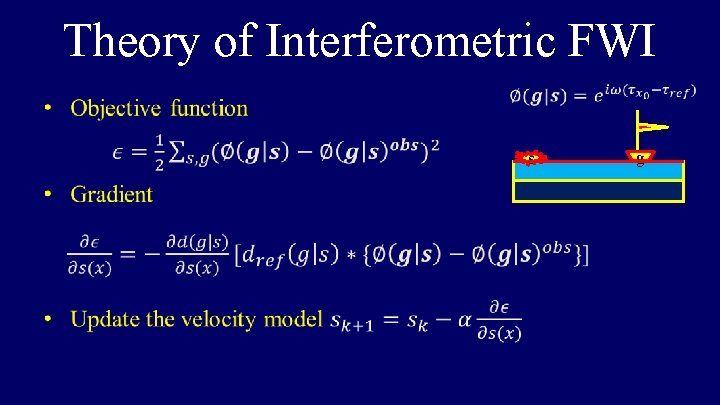
Theory of Interferometric FWI s g

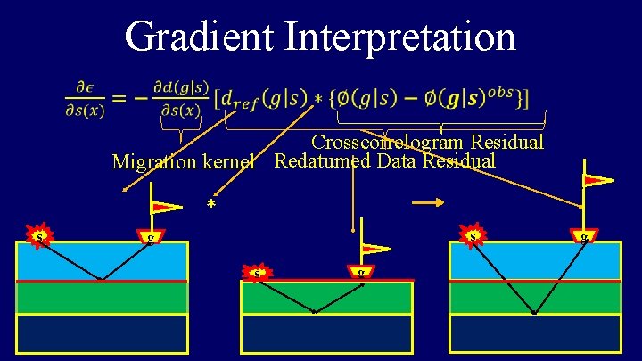
Gradient Interpretation Crosscorrelogram Residual Migration kernel Redatumed Data Residual * s s g g

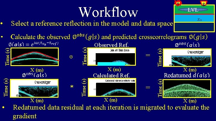
s Workflow • g LVL Select a reference reflection in the model and data space X (m) • * Time (s) X (m) = Calculated Ref. X (m) = X (m) Time (s) ⊗ Observed Ref. Time (s) X (m) Redatumed data residual at each iteration is migrated to evaluate the gradient

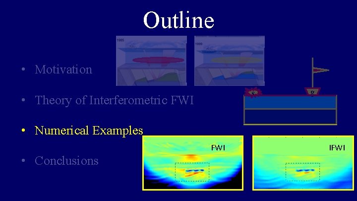
Outline • Motivation s • Theory of Interferometric FWI g • Numerical Examples FWI • Conclusions IFWI

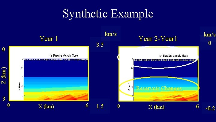
Synthetic Example km/s Year 1 3. 5 0 km/s 0 Year 2 -Year 1 Z (km) Repeatability Errors Reservoir Changes 3 0 X (km) 6 1. 5 0 X (km) 6 -0. 2

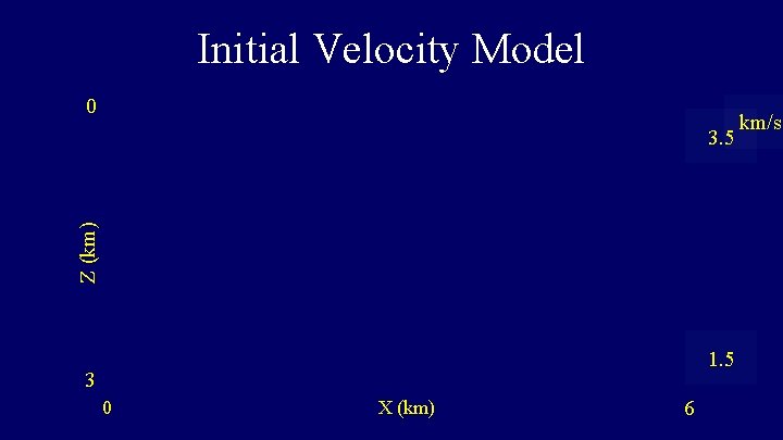
Initial Velocity Model 0 Z (km) 3. 5 1. 5 3 0 X (km) 6 km/s

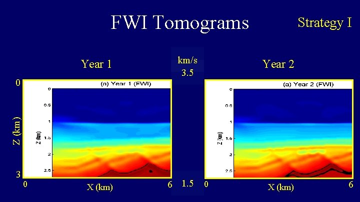
FWI Tomograms Year 1 km/s 3. 5 Year 2 6 1. 5 0 X (km) Z (km) 0 Strategy I 3 0 X (km) 6

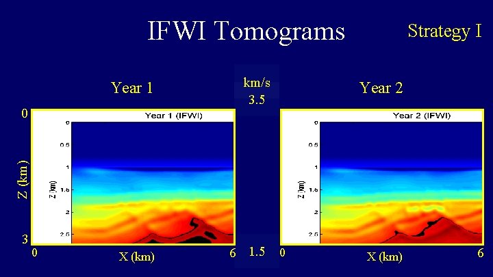
IFWI Tomograms Year 1 km/s 3. 5 Year 2 6 1. 5 0 X (km) Z (km) 0 Strategy I 3 0 X (km) 6

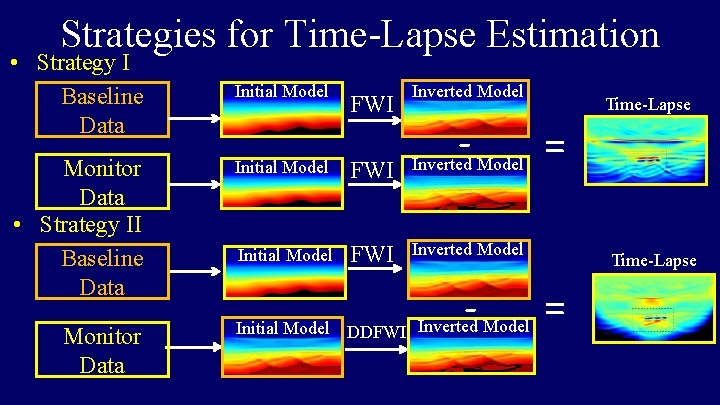
Strategies for Time-Lapse Estimation • Strategy I Baseline Data Monitor Data • Strategy II Baseline Data Monitor Data Initial Model FWI Inverted Model = Inverted Model - Initial Model DDFWI Inverted Model Time-Lapse =

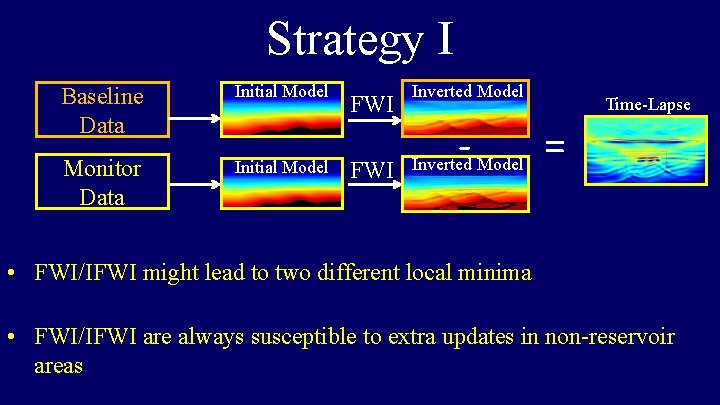
Strategy I Baseline Data Monitor Data Initial Model FWI Inverted Model - Inverted Model Time-Lapse = • FWI/IFWI might lead to two different local minima • FWI/IFWI are always susceptible to extra updates in non-reservoir areas

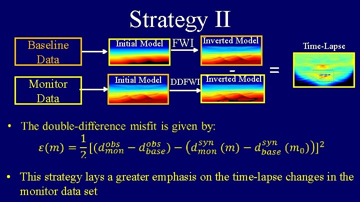
Strategy II FWI Inverted Model Baseline Data Initial Model Monitor Data Initial Model DDFWI Inverted Model - Time-Lapse = • This strategy lays a greater emphasis on the time-lapse changes in the monitor data set

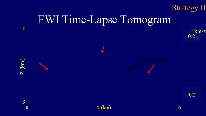
Strategy II FWI Time-Lapse Tomogram 0 km/s 0. 2 Z (km) Reservoir -0. 2 3 0 X (km) 6

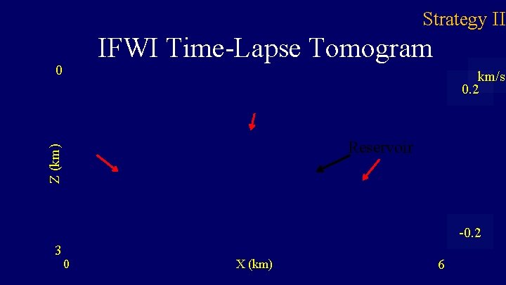
Strategy II IFWI Time-Lapse Tomogram 0 km/s 0. 2 Z (km) Reservoir -0. 2 3 0 X (km) 6

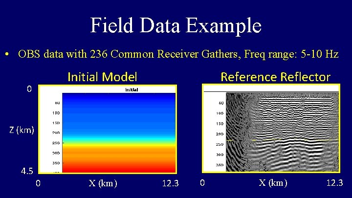
Field Data Example • OBS data with 236 Common Receiver Gathers, Freq range: 5 -10 Hz Initial Model 0 Reference Reflector Z (km) 4. 5 0 X (km) 12. 3

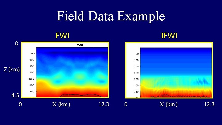
Field Data Example 0 FWI IFWI Z (km) 4. 5 0 X (km) 12. 3

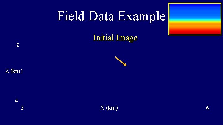
Field Data Example Initial Image 2 Z (km) 4 3 X (km) 6

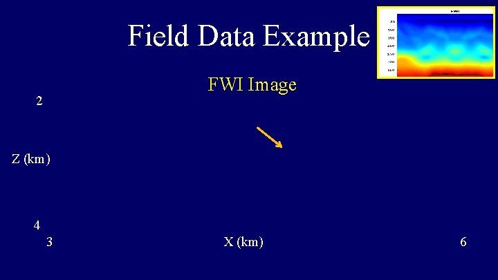
Field Data Example FWI Image 2 Z (km) 4 3 X (km) 6

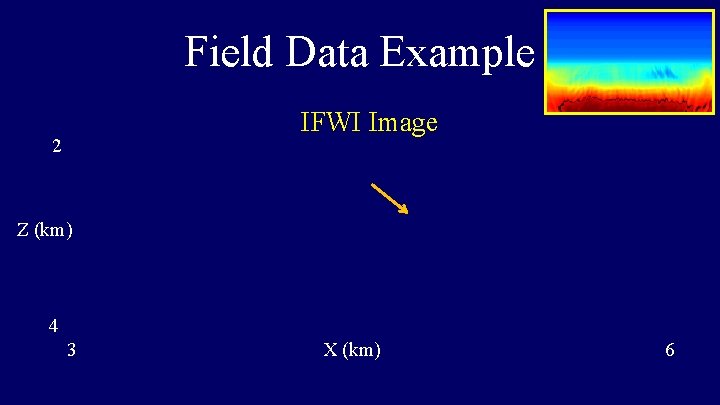
Field Data Example IFWI Image 2 Z (km) 4 3 X (km) 6

Field Data Example Initial Image 2 Z (km) 4 3 X (km) 6

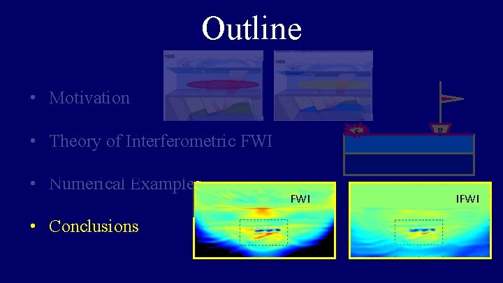
Outline • Motivation s • Theory of Interferometric FWI • Numerical Examples • Conclusions FWI g IFWI

Conclusions • Double-difference IFWI provides a reliable of time-lapse tomogram FWI

Conclusions • Double-difference IFWI provides a reliable of time-lapse tomogram IFWI

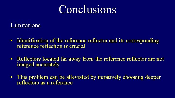
Conclusions Limitations • Identification of the reference reflector and its corresponding reference reflection is crucial • Reflectors located far away from the reference reflector are not imaged accurately • This problem can be alleviated by iteratively choosing deeper reflectors as a reference

Acknowledgements • Sponsors of the CSIM (csim. kaust. edu. sa) consortium. • KAUST Supercomputing Laboratory (KSL) and IT research computing group.

Thank You