Interest Points Computer Vision JiaBin Huang Virginia Tech

Interest Points Computer Vision Jia-Bin Huang, Virginia Tech Many slides from N Snavely, K. Grauman & Leibe, and D. Hoiem

Administrative Stuffs • HW 1 posted, due 11: 59 PM Sept 25 • Submission through Canvas • Frequently Asked Questions for HW 1 will be posted on piazza • Reading - Szeliski: 4. 1

What have we learned so far? • Light and color – What an image records • Filtering in spatial domain • Filtering = weighted sum of neighboring pixels • Smoothing, sharpening, measuring texture • Filtering in frequency domain • Filtering = change frequency of the input image • Denoising, sampling, image compression • Image pyramid and template matching • Filtering = a way to find a template • Image pyramids for coarse-to-fine search and multi -scale detection • Edge detection • Canny edge = smooth -> derivative -> thin -> threshold -> link • Finding straight lines, binary image analysis

This module: Correspondence and Alignment • Correspondence: matching points, patches, edges, or regions across images ≈ Slide credit: Derek Hoiem

This module: Correspondence and Alignment • Alignment/registration: solving the transformation that makes two things match better T Slide credit: Derek Hoiem

The three biggest problems in computer vision? 1. Registration 2. Registration 3. Registration Takeo Kanade (CMU)

Example: automatic panoramas Credit: Matt Brown

Example: fitting an 2 D shape template A Slide from Silvio Savarese

Example: fitting a 3 D object model Slide from Silvio Savarese

Example: estimating “fundamental matrix” that corresponds two views Slide from Silvio Savarese

Example: tracking points x frame 0 x frame 22 x frame 49

Today’s class • What is interest point? • Corner detection • Handling scale and orientation • Feature matching

Why extract features? • Motivation: panorama stitching • We have two images – how do we combine them?

Why extract features? • Motivation: panorama stitching • We have two images – how do we combine them? Step 1: extract features Step 2: match features

Why extract features? • Motivation: panorama stitching • We have two images – how do we combine them? Step 1: extract features Step 2: match features Step 3: align images

Image matching by Diva Sian by swashford

Harder case by Diva Sian by scgbt

Harder still?

Answer below (look for tiny colored squares…) NASA Mars Rover images with SIFT feature matches

Applications • Keypoints are used for: • • • Image alignment 3 D reconstruction Motion tracking Robot navigation Indexing and database retrieval Object recognition

Advantages of local features Locality • features are local, so robust to occlusion and clutter Quantity • hundreds or thousands in a single image Distinctiveness: • can differentiate a large database of objects Efficiency • real-time performance achievable

Overview of Keypoint Matching B 3 A 1 A 2 1. Find a set of distinctive keypoints 2. Define a region around each keypoint A 3 B 2 B 1 3. Extract and normalize the region content 4. Compute a local descriptor from the normalized region 5. Match local descriptors K. Grauman, B. Leibe

Goals for Keypoints Detect points that are repeatable and distinctive

Key trade-offs B 3 A 1 A 2 A 3 B 1 B 2 Detection More Repeatable More Points Robust detection Precise localization Robust to occlusion Works with less texture Description More Distinctive Minimize wrong matches More Flexible Robust to expected variations Maximize correct matches

Choosing interest points Where would you tell your friend to meet you?

Corner Detection: Basic Idea • How does the window change when you shift it? • Shifting the window in any direction causes a big change “flat” region: no change in all directions “edge”: no change along the edge direction “corner”: significant change in all directions Credit: S. Seitz, D. Frolova, D.

Harris corner detection: the math Consider shifting the window W by (u, v) • how do the pixels in W change? • compare each pixel before and after by summing up the squared differences (SSD) • this defines an SSD “error” E(u, v): W

Small motion assumption Taylor Series expansion of I: If the motion (u, v) is small, then first order approximation is good Plugging this into the formula on the previous slide…

Harris corner detection: the math Using the small motion assumption, replace I with a linear approximation (Shorthand: ) W

Corner detection: the math W • Thus, E(u, v) is locally approximated as a quadratic form

The second moment matrix The surface E(u, v) is locally approximated by a quadratic form. Let’s try to understand its shape.

E(u, v) Horizontal edge: u v

E(u, v) Vertical edge: u v

General case The shape of H tells us something about the distribution of gradients around a pixel We can visualize H as an ellipse with axis lengths determined by the eigenvalues of H and orientation determined by the eigenvectors of H Ellipse equation: direction of the fastest change max, min : eigenvalues of H direction of the slowest change ( max)-1/2 ( min)-1/2

Quick eigenvalue/eigenvector review The eigenvectors of a matrix A are the vectors x that satisfy: The scalar is the eigenvalue corresponding to x • The eigenvalues are found by solving: • In our case, A = H is a 2 x 2 matrix, so we have • The solution: Once you know , you find x by solving

Corner detection: the math xmin xmax Eigenvalues and eigenvectors of H • Define shift directions with the smallest and largest change in error • xmax = direction of largest increase in E • max = amount of increase in direction xmax • xmin = direction of smallest increase in E • min = amount of increase in direction xmin

Corner detection: the math How are max, xmax, min, and xmin relevant for feature detection? • What’s our feature scoring function?

Corner detection: the math How are max, xmax, min, and xmin relevant for feature detection? • What’s our feature scoring function? Want E(u, v) to be large for small shifts in all directions • the minimum of E(u, v) should be large, over all unit vectors [u v] • this minimum is given by the smaller eigenvalue ( min) of H

Interpreting the eigenvalues Classification of image points using eigenvalues of M: 2 “Edge” 2 >> 1 “Corner” 1 and 2 are large, 1 ~ 2; E increases in all directions 1 and 2 are small; E is almost constant in all directions “Flat” region “Edge” 1 >> 2 1

Corner detection summary Here’s what you do • Compute the gradient at each point in the image • Create the H matrix from the entries in the gradient • Compute the eigenvalues. • Find points with large response ( min > threshold) • Choose those points where min is a local maximum as features

The Harris operator min is a variant of the “Harris operator” for feature detection • • The trace is the sum of the diagonals, i. e. , trace(H) = h 11 + h 22 Very similar to min but less expensive (no square root) Called the “Harris Corner Detector” or “Harris Operator” Lots of other detectors, this is one of the most popular

The Harris operator

Harris detector example

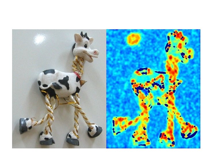
f value (red high, blue low)

Threshold (f > value)

Find local maxima of f

Harris features (in red)

Weighting the derivatives • In practice, using a simple window W doesn’t work too well • Instead, we’ll weight each derivative value based on its distance from the center pixel

Harris Detector – Responses [Harris 88] Effect: A very precise corner detector.

Harris Detector – Responses [Harris 88]

Harris Detector: Invariance Properties • Rotation Ellipse rotates but its shape (i. e. eigenvalues) remains the same Corner response is invariant to image rotation

Harris Detector: Invariance Properties • Affine intensity change: I a. I + b ü Only derivatives are used => invariance to intensity shift I I + b ü Intensity scale: I a I R R threshold x (image coordinate) Partially invariant to affine intensity change

Harris Detector: Invariance Properties • Scaling Corner All points will be classified as edges Not invariant to scaling

Scale invariant detection Suppose you’re looking for corners Key idea: find scale that gives local maximum of f • in both position and scale • One definition of f: the Harris operator

Automatic Scale Selection How to find corresponding patch sizes? K. Grauman, B. Leibe

Automatic Scale Selection • Function responses for increasing scale (scale signature) K. Grauman, B. Leibe

Implementation • Instead of computing f for larger and larger windows, we can implement using a fixed window size with a Gaussian pyramid (sometimes need to create inbetween levels, e. g. a ¾-size image)

What Is A Useful Signature Function? • Difference-of-Gaussian = “blob” detector K. Grauman, B. Leibe

Difference-of-Gaussian (Do. G) = K. Grauman, B. Leibe

Do. G – Efficient Computation • Computation in Gaussian scale pyramid Sampling with step s 4 =2 s s s Original image s K. Grauman, B. Leibe

Find local maxima in position-scale space of Difference-of-Gaussian s 5 s 4 s 3 s 2 List of s K. Grauman, B. Leibe (x, y, s)

Results: Difference-of-Gaussian K. Grauman, B. Leibe

Orientation Normalization [Lowe, SIFT, 1999] • Compute orientation histogram • Select dominant orientation • Normalize: rotate to fixed orientation 0 T. Tuytelaars, B. Leibe 2

Maximally Stable Extremal Regions • Based on Watershed segmentation algorithm • Select regions that stay stable over a large parameter range K. Grauman, B. Leibe [Matas ‘ 02]

Example Results: MSER 73 K. Grauman, B. Leibe

Available at a web site near you… • For most local feature detectors, executables are available online: – http: //www. robots. ox. ac. uk/~vgg/research/affine – http: //www. cs. ubc. ca/~lowe/keypoints/ – http: //www. vision. ee. ethz. ch/~surf K. Grauman, B. Leibe

Local Descriptors • The ideal descriptor should be – Robust – Distinctive – Compact – Efficient • Most available descriptors focus on edge/gradient information – Capture texture information – Color rarely used K. Grauman, B. Leibe

Scale Invariant Feature Transform Basic idea: • • Take 16 x 16 square window around detected feature Compute edge orientation (angle of the gradient - 90 ) for each pixel Throw out weak edges (threshold gradient magnitude) Create histogram of surviving edge orientations 0 2 angle histogram Adapted from slide by David Lowe

SIFT descriptor Full version • Divide the 16 x 16 window into a 4 x 4 grid of cells (2 x 2 case shown below) • Compute an orientation histogram for each cell • 16 cells * 8 orientations = 128 dimensional descriptor Adapted from slide by David Lowe

Local Descriptors: SIFT Descriptor [Lowe, ICCV 1999] Histogram of oriented gradients • Captures important texture information • Robust to small translations / affine deformations K. Grauman, B. Leibe

Details of Lowe’s SIFT algorithm • Run Do. G detector – Find maxima in location/scale space – Remove edge points • Find all major orientations – Bin orientations into 36 bin histogram • Weight by gradient magnitude • Weight by distance to center (Gaussian-weighted mean) – Return orientations within 0. 8 of peak • Use parabola for better orientation fit • For each (x, y, scale, orientation), create descriptor: – – Sample 16 x 16 gradient mag. and rel. orientation Bin 4 x 4 samples into 4 x 4 histograms Threshold values to max of 0. 2, divide by L 2 norm Final descriptor: 4 x 4 x 8 normalized histograms Lowe IJCV 2004

SIFT Example sift 868 SIFT features

Feature matching Given a feature in I 1, how to find the best match in I 2? 1. Define distance function that compares two descriptors 2. Test all the features in I 2, find the one with min distance

Feature distance How to define the difference between two features f 1, f 2? • • Simple approach: L 2 distance, ||f 1 - f 2 || can give good scores to ambiguous (incorrect) matches f 1 f 2 I 1 I 2

Feature distance How to define the difference between two features f 1, f 2? • Better approach: ratio distance = ||f 1 - f 2 || / || f 1 - f 2’ || • f 2 is best SSD match to f 1 in I 2 • f 2’ is 2 nd best SSD match to f 1 in I 2 • gives large values for ambiguous matches f 1 f 2' I 1 I 2 f 2

Feature matching example 51 matches

Feature matching example 58 matches

Evaluating the results How can we measure the performance of a feature matcher? 50 75 200 feature distance

True/false positives How can we measure the performance of a feature matcher? 50 75 true match 200 false match feature distance The distance threshold affects performance • True positives = # of detected matches that are correct • Suppose we want to maximize these—how to choose threshold? • False positives = # of detected matches that are incorrect • Suppose we want to minimize these—how to choose threshold?

Evaluating the results How can we measure the performance of a feature matcher? 1 0. 7 # true positives # correctly matched features (positives) true positive rate “recall” 0 0. 1 false positive rate 1 # false positives # incorrectly matched features (negatives) 1 - “precision”

Evaluating the results How can we measure the performance of a feature matcher? 1 ROC curve (“Receiver Operator Characteristic”) 0. 7 # true positives # correctly matched features (positives) true positive rate “recall” 0 0. 1 false positive rate 1 # false positives # incorrectly matched features (negatives) 1 - “precision”

Matching SIFT Descriptors • Nearest neighbor (Euclidean distance) • Threshold ratio of nearest to 2 nd nearest descriptor Lowe IJCV 2004

SIFT Repeatability Lowe IJCV 2004

SIFT Repeatability

SIFT Repeatability Lowe IJCV 2004

Local Descriptors: SURF • Fast approximation of SIFT idea Ø Ø Efficient computation by 2 D box filters & integral images 6 times faster than SIFT Equivalent quality for object identification • GPU implementation available Many other efficient descriptors are also available Ø Ø [Bay, ECCV’ 06], [Cornelis, CVGPU’ 08] Feature extraction @ 200 Hz (detector + descriptor, 640× 480 img) http: //www. vision. ee. ethz. ch/~surf K. Grauman, B. Leibe

Local Descriptors: Shape Context Count the number of points inside each bin, e. g. : Count = 4. . . Count = 10 Log-polar binning: more precision for nearby points, more flexibility for farther points. Belongie & Malik, ICCV 2001 K. Grauman, B. Leibe

Local Descriptors: Geometric Blur Compute edges at four orientations Extract a patch in each channel ~ Apply spatially varying blur and sub-sample Example descriptor (Idealized signal) Berg & Malik, CVPR 2001 K. Grauman, B. Leibe

Choosing a detector • What do you want it for? – Precise localization in x-y: Harris – Good localization in scale: Difference of Gaussian – Flexible region shape: MSER • Best choice often application dependent – Harris-/Hessian-Laplace/Do. G work well for many natural categories – MSER works well for buildings and printed things • Why choose? – Get more points with more detectors • There have been extensive evaluations/comparisons – [Mikolajczyk et al. , IJCV’ 05, PAMI’ 05] – All detectors/descriptors shown here work well

Comparison of Keypoint Detectors Tuytelaars Mikolajczyk 2008

Choosing a descriptor • Again, need not stick to one • For object instance recognition or stitching, SIFT or variant is a good choice

Recent advances in interest points Features from Accelerated Segment Test, ECCV 06 Binary feature descriptors • • • BRIEF: Binary Robust Independent Elementary Features, ECCV 10 ORB (Oriented FAST and Rotated BRIEF), CVPR 11 BRISK: Binary robust invariant scalable keypoints, ICCV 11 Freak: Fast retina keypoint, CVPR 12 LIFT: Learned Invariant Feature Transform, ECCV 16

Things to remember • Keypoint detection: repeatable and distinctive • Corners, blobs, stable regions • Harris, Do. G • Descriptors: robust and selective • spatial histograms of orientation • SIFT

Open. CV demo – Feature Detection

Thank you • Next class: feature tracking and optical flow