Interest Points and Harris Corner Detector Slide credits

Interest Points and Harris Corner Detector Slide credits: James Tompkin, Rick Szeliski, Svetlana Lazebnik, Derek Hoiem and Grauman&Leibe

Filtering Edges Corners Feature points Also called interest points, key points, etc. Often described as ‘local’ features. Szeliski 4. 1 Slides from Rick Szeliski, Svetlana Lazebnik, Derek Hoiem and Grauman&Leibe 2008 AAAI Tutorial

Correspondence across views • Correspondence: matching points, patches, edges, or regions across images. ≈ Hays

Example: estimate “fundamental matrix” that corresponds two views Silvio Savarese

Example: structure from motion

Fundamental to Applications • Feature points are used for: – – – Image alignment 3 D reconstruction Motion tracking (robots, drones, AR) Indexing and database retrieval Object recognition … Hays

Example: Invariant Local Features Detect points that are repeatable and distinctive. I. E. , invariant to image transformations: - appearance variation (brightness, illumination) - geometric variation (translation, rotation, scale). Keypoint Descriptors James Hays

Example application • Panorama stitching • We have two images – how do we combine them?

Local features: main components 1) Detection: Find a set of distinctive key points. 2) Description: Extract feature descriptor around each interest point as vector. 3) Matching: Compute distance between feature vectors to find correspondence. K. Grauman, B. Leibe

Characteristics of good features • Repeatability • The same feature can be found in several images despite geometric and photometric transformations • Saliency • Each feature is distinctive • Compactness and efficiency • Many fewer features than image pixels • Locality • A feature occupies a relatively small area of the image; robust to clutter and occlusion Kristen Grauman

Goal: interest operator repeatability • We want to detect (at least some of) the same points in both images. With these points, there’s no chance to find true matches! • Yet we have to be able to run the detection procedure independently per image. Kristen Grauman

Goal: descriptor distinctiveness • We want to be able to reliably determine which point goes with which. ? • Must provide some invariance to geometric and photometric differences between the two views. Kristen Grauman

Local features: main components 1) Detection: Find a set of distinctive key points. 2) Description: Extract feature descriptor around each interest point as vector. 3) Matching: Compute distance between feature vectors to find correspondence. Comparing with edges and “flat” regions, corners are more unique

Corner Detection: Basic Idea • We might recognize the point by looking through a small window. • We want a window shift in any direction to give a large change in intensity. “Flat” region: no change in all directions “Edge”: no change along the edge direction “Corner”: significant change in all directions A. Efros

Corner Detection by Auto-correlation Change in appearance of window w(x, y) for shift [u, v]: Window function Shifted intensity Window function w(x, y) = Intensity or 1 in window, 0 outside Gaussian Source: R. Szeliski

Corner Detection by Auto-correlation Change in appearance of window w(x, y) for shift [u, v]: Window function Shifted intensity Intensity Warning: sloppy notation! Probably should write Source: R. Szeliski

Fun time: Correspond the three red crosses to (b, c, d). As a surface

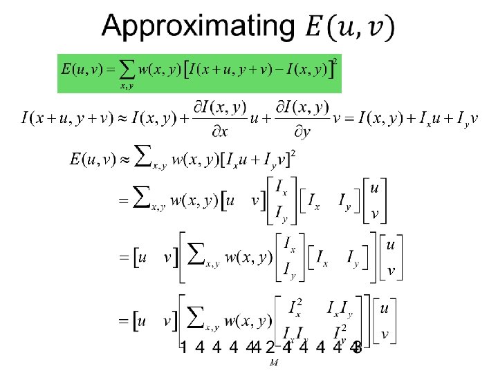
Corner Detection by Auto-correlation Change in appearance of window w(x, y) for shift [u, v]: We want to discover how E behaves for small shifts But this is very slow to compute naively. O(window_width 2 * shift_range 2 * image_width 2) O( 112 * 6002 ) = 5. 2 billion of these 14. 6 thousand per pixel in your image

Corner Detection by Auto-correlation Change in appearance of window w(x, y) for shift [u, v]: We want to discover how E behaves for small shifts Can speed up using Tayler series expansion

Recall: Taylor series expansion A function f can be represented by an infinite series of its derivatives at a single point a: Wikipedia As we care about window centered, we set a = 0 (Mac. Laurin series) Approximation of f(x) = ex centered at f(0)

Corner Detection: Mathematics The quadratic approximation simplifies to where M is a second moment matrix computed from image derivatives:

Corners as distinctive interest points 2 x 2 matrix of image derivatives (averaged in neighborhood of a point) Notation: James Hays

Interpreting the second moment matrix The surface E(u, v) is locally approximated by a quadratic form. Let’s try to understand its shape. James Hays

Interpreting the second moment matrix Consider a horizontal “slice” of E(u, v): This is the equation of an ellipse. Recall that E(u, v) is the square difference between shifted patch and itself James Hays

Eigenvector and eigenvalue 1. Scaled eigenvector is still eigenvector with same eigenvalue 2. Eigenvectors diagonalize the matrix

Eigenvector and eigenvalue 3. For symmetric M, R can be made orthonormal (orthogonal and normalized) • • In particular, if (try at home) R orthonormal R is a rotation operation 4. E(u, v) = 1 is a rotated eclipse (by R)

Interpreting the second moment matrix ( max)-1/2 ( min)-1/2 direction of the fastest change direction of the slowest change ( max)-1/2 ( min)-1/2 James Hays

Fun time ( max)-1/2 ( min)-1/2 Flat region Corner Edge

Classification of image points using eigenvalues of M 2 “Edge” 2 >> 1 “Corner” 1 and 2 are large, 1 ~ 2; E increases in all directions 1 and 2 are small; E is almost constant in all directions “Flat” region “Edge” 1 >> 2 1

Classification of image points using eigenvalues of M Cornerness 2 “Edge” C<0 α: constant (0. 04 to 0. 06) “Corner” C>0 |C| small “Flat” region “Edge” C<0 1

Classification of image points using eigenvalues of M Cornerness 2 “Edge” C<0 α: constant (0. 04 to 0. 06) “Corner” C>0 |C| small “Flat” region “Edge” C<0 1

Classification of image points using eigenvalues of M Cornerness 2 “Edge” C<0 α: constant (0. 04 to 0. 06) “Corner” C>0 Remember your linear algebra: Determinant: Trace: |C| small “Flat” region “Edge” C<0 1

Harris corner detector C. Harris and M. Stephens. “A Combined Corner and Edge Detector. ” Proceedings of the 4 th Alvey Vision Conference: pages 147— 151, 1988.

Harris Corner Detector [Harris 88] James Hays 0. Input image We want to compute M at each pixel. 1. Compute image derivatives (optionally, blur first). 3. Gaussian filter g() with width s 4. Compute cornerness

Harris Detector: Steps

Harris Detector: Steps

Harris Detector: Steps

Harris Detector: Steps

Harris Detector: Steps

Invariance and covariance Are locations invariant to photometric transformations and covariant to geometric transformations? • Invariance: image is transformed and corner locations do not change • Covariance: if we have two transformed versions of the same image, features should be detected in corresponding locations

Shi-Tomashi corner detector • Just a slight variation of Harris corner detector • Instead of having as criterion. We have instead

Conclusion • Key point, interest point, local feature detection is a staple in computer vision. Uses such as • • • Image alignment 3 D reconstruction Motion tracking (robots, drones, AR) Indexing and database retrieval Object recognition • Harris corner detection is one classic example • More key point detection techniques next time