Interactive Methods in Scientific Visualization Interactive Methods in

Interactive Methods in Scientific Visualization

Interactive Methods in Scientific Visualization Jens Schneider

Large Data Vis - Disambiguation • What we won’t cover • Parallel rendering / visualization • What we will cover • • Management of large data Compression of large data Paging strategies Multicore-optimizations

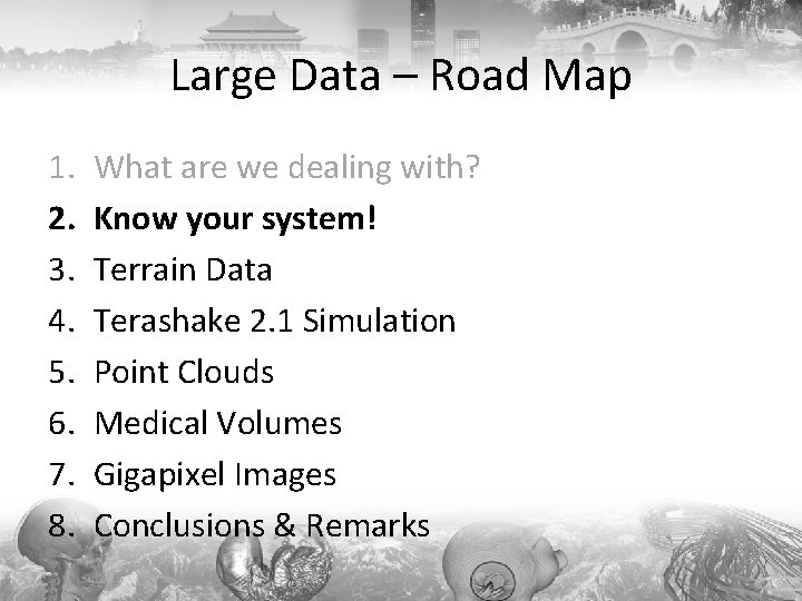
Large Data – Road Map 1. 2. 3. 4. 5. 6. 7. 8. What are we dealing with? Know your system! Terrain Data Terashake 2. 1 Simulation Point Clouds Medical Volumes Gigapixel Images Conclusions & Remarks

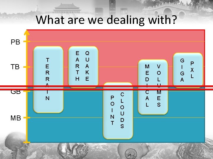
What are we dealing with? PB TB GB MB T E R R A I N E A R T H Q U A K E P O I N T C L O U D S M E D I C A L V O L U M E S G I G A P X L

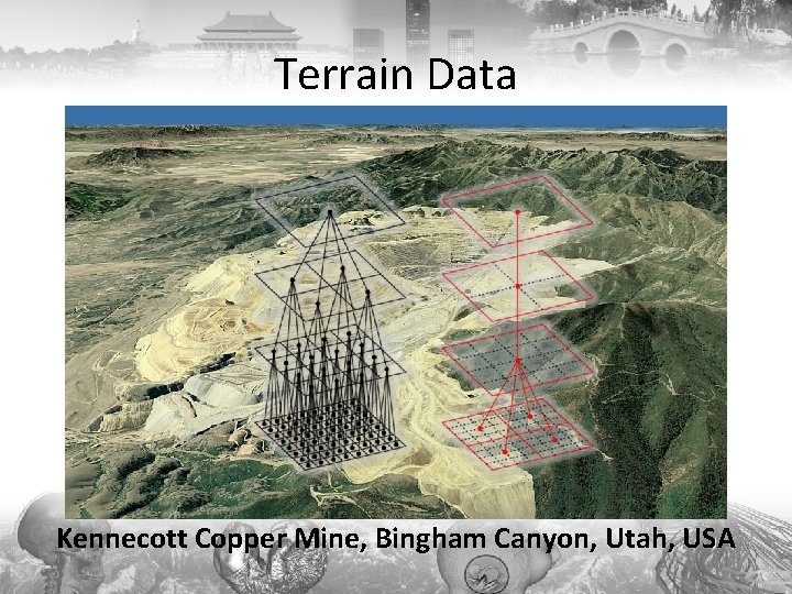
Terrain Data Kennecott Copper Mine, Bingham Canyon, Utah, USA

Earth Quake Simulation SDSC Terashake 2. 1, Palm Springs & L. A. , CA, USA

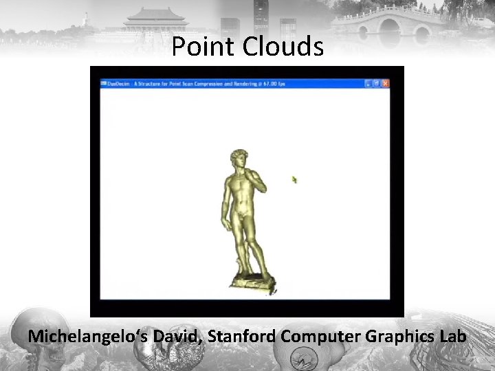
Point Clouds Michelangelo‘s David, Stanford Computer Graphics Lab

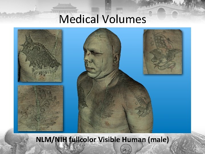
Medical Volumes NLM/NIH fullcolor Visible Human (male)

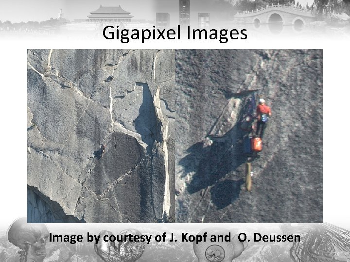
Gigapixel Images Image by courtesy of J. Kopf and O. Deussen

Large Data – Road Map 1. 2. 3. 4. 5. 6. 7. 8. What are we dealing with? Know your system! Terrain Data Terashake 2. 1 Simulation Point Clouds Medical Volumes Gigapixel Images Conclusions & Remarks

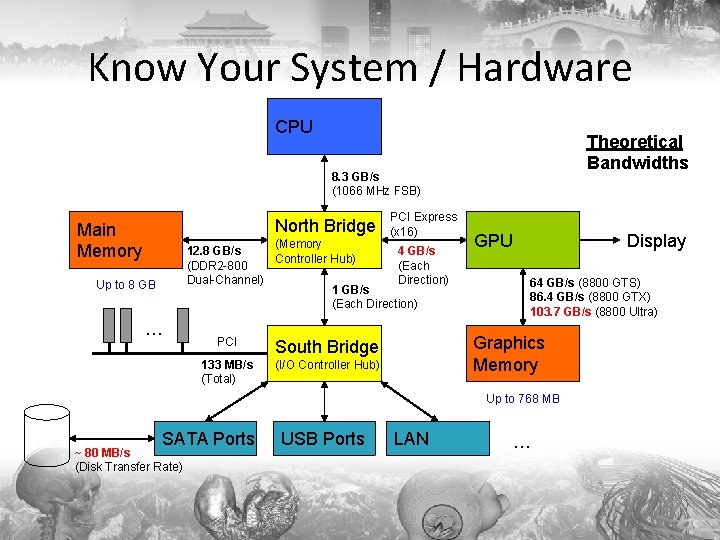
Know Your System / Hardware CPU Theoretical Bandwidths 8. 3 GB/s (1066 MHz FSB) North Bridge Main Memory PCI Express (x 16) (Memory 12. 8 GB/s 4 GB/s Controller Hub) (DDR 2 -800 (Each Dual-Channel) Direction) 1 GB/s (Each Direction) Up to 8 GB … PCI South Bridge 133 MB/s (Total) (I/O Controller Hub) Display GPU 64 GB/s (8800 GTS) 86. 4 GB/s (8800 GTX) 103. 7 GB/s (8800 Ultra) Graphics Memory Up to 768 MB SATA Ports ~ 80 MB/s (Disk Transfer Rate) USB Ports LAN …

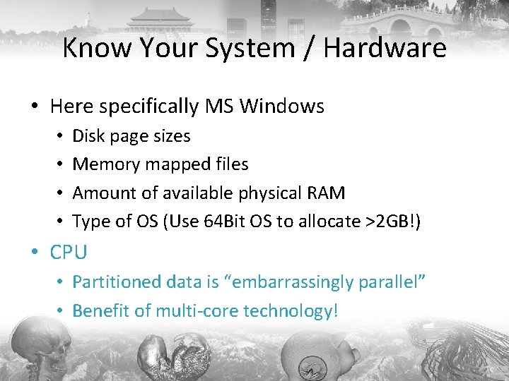
Know Your System / Hardware • Here specifically MS Windows • • Disk page sizes Memory mapped files Amount of available physical RAM Type of OS (Use 64 Bit OS to allocate >2 GB!) • CPU • Partitioned data is “embarrassingly parallel” • Benefit of multi-core technology!

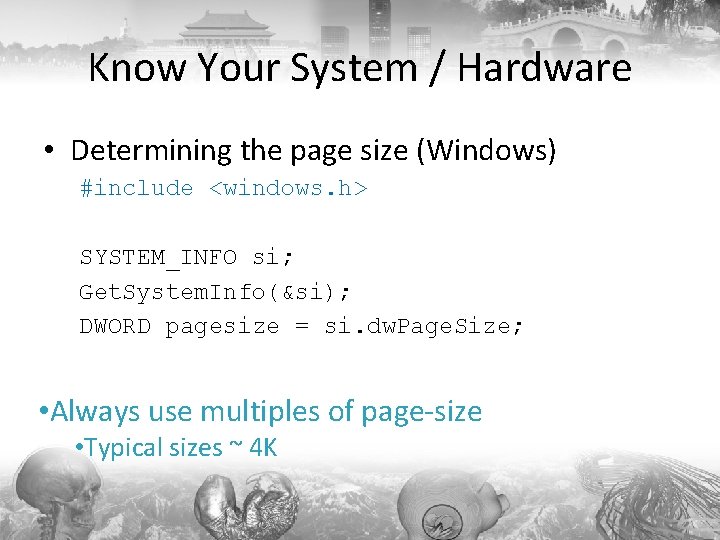
Know Your System / Hardware • Determining the page size (Windows) #include <windows. h> SYSTEM_INFO si; Get. System. Info(&si); DWORD pagesize = si. dw. Page. Size; • Always use multiples of page-size • Typical sizes ~ 4 K

Know Your System / Hardware • Determining amt. of physical RAM (Windows) #include<windows. h> MEMORYSTATUS mem. Info; mem. Info. dw. Length = sizeof(mem. Info); Global. Memory. Status(&mem. Info); size_t avail. Bytes = mem. Info. dw. Avail. Phys; • Allocate 60% - 75% at initialization • Dynamic allocation / release affects performance!

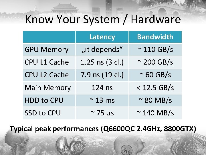
Know Your System / Hardware Latency Bandwidth GPU Memory „it depends“ ~ 110 GB/s CPU L 1 Cache 1. 25 ns (3 cl. ) ~ 200 GB/s CPU L 2 Cache 7. 9 ns (19 cl. ) ~ 60 GB/s Main Memory 124 ns < 12. 5 GB/s HDD to CPU ~ 13 ms ~ 80 MB/s SSD to CPU ~ 75 µs ~ 140 MB/s Typical peak performances (Q 6600 QC 2. 4 GHz, 8800 GTX)

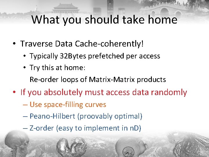
What you should take home • Traverse Data Cache-coherently! • Typically 32 Bytes prefetched per access • Try this at home: Re-order loops of Matrix-Matrix products • If you absolutely must access data randomly – Use space-filling curves – Peano-Hilbert (proovably optimal) – Z-order (easy to implement in n. D)

Large Data – Road Map 1. 2. 3. 4. 5. 6. 7. 8. What are we dealing with? Know your system! Terrain Data Terashake 2. 1 Simulation Point Clouds Medical Volumes Gigapixel Images Conclusions & Remarks

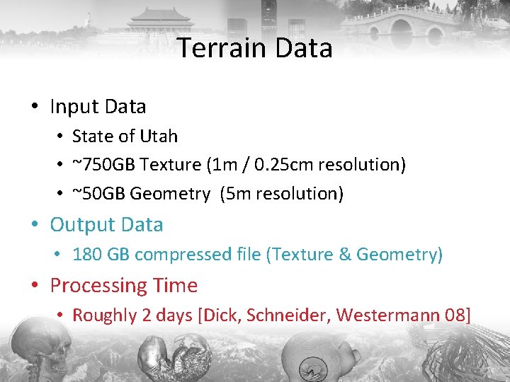
Terrain Data • Input Data • State of Utah • ~750 GB Texture (1 m / 0. 25 cm resolution) • ~50 GB Geometry (5 m resolution) • Output Data • 180 GB compressed file (Texture & Geometry) • Processing Time • Roughly 2 days [Dick, Schneider, Westermann 08]

Terrain Data • Methods • • • Merging of different resolutions (out-of-core) Clipmap generation (out-of-core) Data tiling (implicitly) S 3 TC (in-core, still expensive) Geometry compression (in-core, cheap) • Use of 64 Bit Addressing (up to 16384 PB) • size_t gets promoted automatically! • Paging, Streaming, Multi-core architectures

Terrain Data - Methods • Tiles may come in different resolutions • Need uniform resolution for rendering • Use splatting to combine them • Large 2 D Array abstraction • • Behave like C-Arrays Memory mapped file wrapper Process data logical-page-wise! (here: 4 MB) Code: http: //wwwcg. in. tum. de/Tutorials

Terrain Data - Methods • Merging resolutions • • • Store pair<float, float> in 2 D array Choose radius around sample wrt resolution Use Gaussian weights Second pass normalizes Caveat: May blur the data, but fast! • Clipmap Generation • Successive box filtering, to another large array

Terrain Data - Methods • Geometry Compression: Christian Dick • Data Tiling • Gather full 5122 mipmaps from various files • S 3 Texture Compression – About 0. 5 s for 5122 [Simon Brown’s Squish Lib] – Good speed-up on multi-cores (3. 7 x on 4 cores) – Reason: Almost sync-free – Recommendation: Use intel’s TBB Lib.

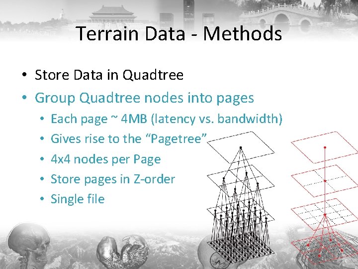
Terrain Data - Methods • Store Data in Quadtree • Group Quadtree nodes into pages • • • Each page ~ 4 MB (latency vs. bandwidth) Gives rise to the “Pagetree” 4 x 4 nodes per Page Store pages in Z-order Single file

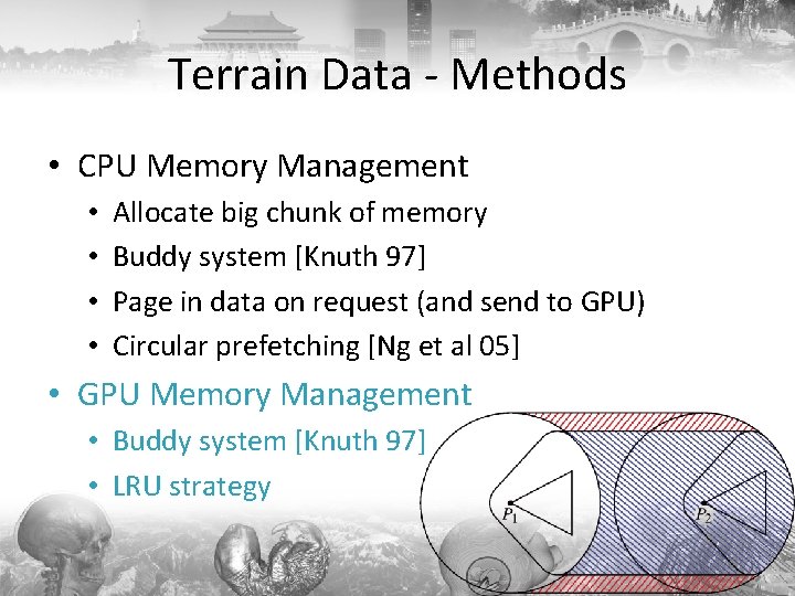
Terrain Data - Methods • CPU Memory Management • • Allocate big chunk of memory Buddy system [Knuth 97] Page in data on request (and send to GPU) Circular prefetching [Ng et al 05] • GPU Memory Management • Buddy system [Knuth 97] • LRU strategy

Large Data – Road Map 1. 2. 3. 4. 5. 6. 7. 8. What are we dealing with? Know your system! Terrain Data Terashake 2. 1 Simulation Point Clouds Medical Volumes Gigapixel Images Conclusions & Remarks

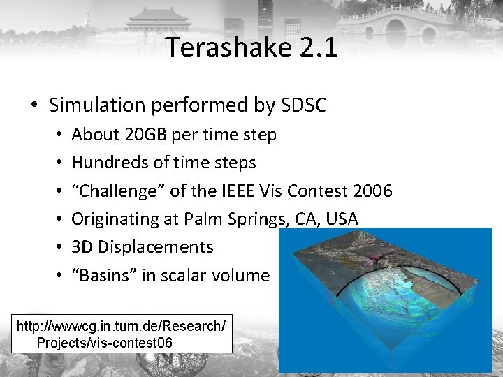
Terashake 2. 1 • Simulation performed by SDSC • • • About 20 GB per time step Hundreds of time steps “Challenge” of the IEEE Vis Contest 2006 Originating at Palm Springs, CA, USA 3 D Displacements “Basins” in scalar volume http: //wwwcg. in. tum. de/Research/ Projects/vis-contest 06

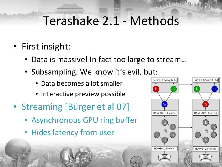
Terashake 2. 1 - Methods • First insight: • Data is massive! In fact too large to stream… • Subsampling. We know it‘s evil, but: • Data becomes a lot smaller • Interactive preview possible • Streaming [Bürger et al 07] • Asynchronous GPU ring buffer • Hides latency from user

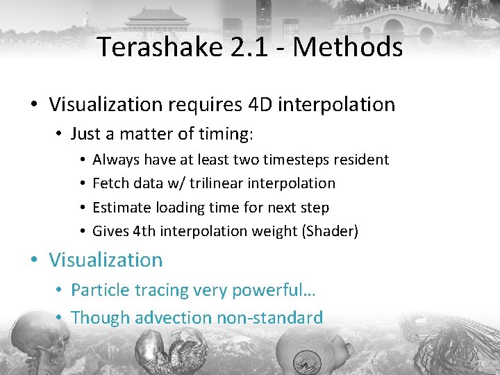
Terashake 2. 1 - Methods • Visualization requires 4 D interpolation • Just a matter of timing: • • Always have at least two timesteps resident Fetch data w/ trilinear interpolation Estimate loading time for next step Gives 4 th interpolation weight (Shader) • Visualization • Particle tracing very powerful… • Though advection non-standard

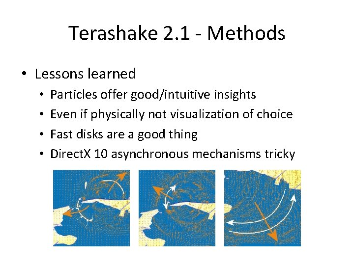
Terashake 2. 1 - Methods • Lessons learned • • Particles offer good/intuitive insights Even if physically not visualization of choice Fast disks are a good thing Direct. X 10 asynchronous mechanisms tricky

Large Data – Road Map 1. 2. 3. 4. 5. 6. 7. 8. What are we dealing with? Know your system! Terrain Data Terashake 2. 1 Simulation Point Clouds Medical Volumes Gigapixel Images Conclusions & Remarks

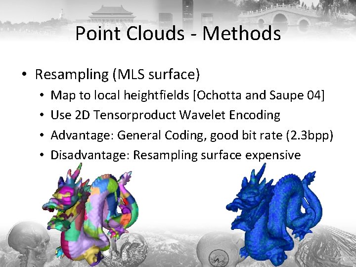
Point Clouds - Methods • Resampling (MLS surface) • • Map to local heightfields [Ochotta and Saupe 04] Use 2 D Tensorproduct Wavelet Encoding Advantage: General Coding, good bit rate (2. 3 bpp) Disadvantage: Resampling surface expensive

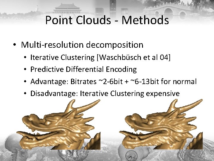
Point Clouds - Methods • Multi-resolution decomposition • • Iterative Clustering [Waschbüsch et al 04] Predictive Differential Encoding Advantage: Bitrates ~2 -6 bit + ~6 -13 bit for normal Disadvantage: Iterative Clustering expensive

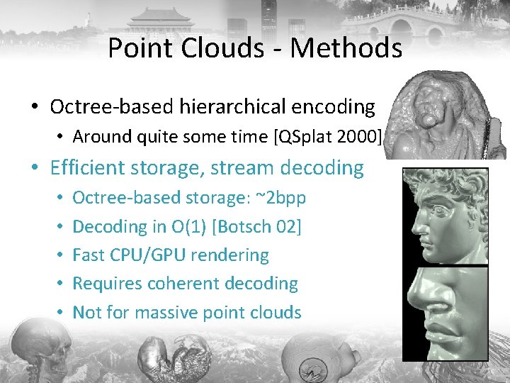
Point Clouds - Methods • Octree-based hierarchical encoding • Around quite some time [QSplat 2000] • Efficient storage, stream decoding • • • Octree-based storage: ~2 bpp Decoding in O(1) [Botsch 02] Fast CPU/GPU rendering Requires coherent decoding Not for massive point clouds

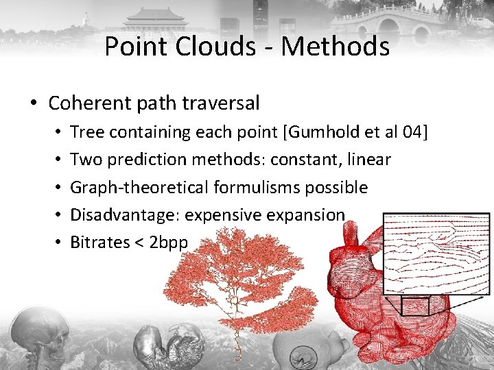
Point Clouds - Methods • Coherent path traversal • • • Tree containing each point [Gumhold et al 04] Two prediction methods: constant, linear Graph-theoretical formulisms possible Disadvantage: expensive expansion Bitrates < 2 bpp

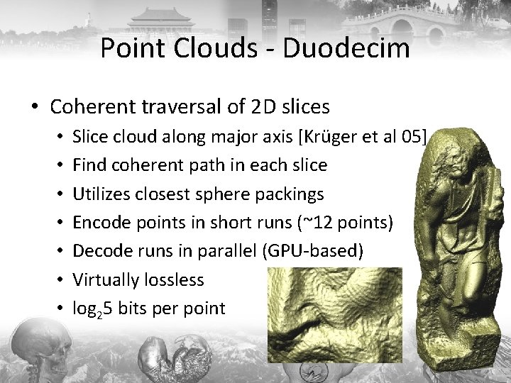
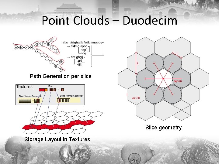
Point Clouds - Duodecim • Coherent traversal of 2 D slices • • Slice cloud along major axis [Krüger et al 05] Find coherent path in each slice Utilizes closest sphere packings Encode points in short runs (~12 points) Decode runs in parallel (GPU-based) Virtually lossless log 25 bits per point

Point Clouds - Duodecim • Sort points along major axis • Out-of-core sorting [Sedgewick 98] • “Slab” points perpendicular to major axis • • • Efficient stream operation on sorted points! Grid points per slab into hexagonal grid Find spanning tree between connected points Convert tree into path Encode differentially

Point Clouds – Duodecim Path Generation per slice Slice geometry Storage Layout in Textures

Point Clouds - Duodecim • GPU-based decoding • • • Page in required textures (driver-based paging) Decode runs in parallel (requires state!) Write decoded positions & normals to vertex array Render vertex array High Quality rendering [Botsch 03, Krüger 06] • LOD based on multires hierarchy • Introduces storage overhead

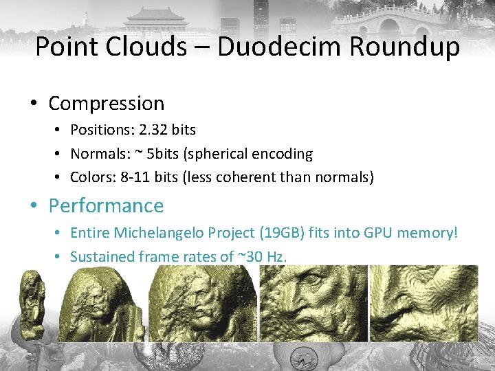
Point Clouds – Duodecim Roundup • Compression • Positions: 2. 32 bits • Normals: ~ 5 bits (spherical encoding • Colors: 8 -11 bits (less coherent than normals) • Performance • Entire Michelangelo Project (19 GB) fits into GPU memory! • Sustained frame rates of ~30 Hz.

Large Data – Road Map 1. 2. 3. 4. 5. 6. 7. 8. What are we dealing with? Know your system! Terrain Data Terashake 2. 1 Simulation Point Clouds Medical Volumes Gigapixel Images Conclusions & Remarks

Medical Volumes • Bricking is a trivial task – or isn‘t it? • Bricks can be paged and rendered separately • Observe rendering order for blending • Generating Multi-res representation • • • Generally not trivial! Successive box filtering will blur the data Feature Preserving methods Metrics that preserve appearance Use any method you trust (details not discussed here)

Medical Volumes • Rendering: Christof Rezk-Salama • Memory Management • Example: Image. Vis 3 D, SCI, University of Utah • Paging of Bricks using tightest-fit re-use of blocks • If one (of many) tightest fitting blocks is found, use MRU (!) • Rationale behind MRU – LRU results in excessive paging if RAM scarce – Reason: Entire data set will be paged each frame!

Large Data – Road Map 1. 2. 3. 4. 5. 6. 7. 8. What are we dealing with? Know your system! Terrain Data Terashake 2. 1 Simulation Point Clouds Medical Volumes Gigapixel Images Conclusions & Remarks

Gigapixel Images • Original Paper by Kopf et al [2007] • Discusses Acquisition: • Multi-camera snapshots, color matching, stitching • And Rendering: • HDR, perspective, etc. • Alternative: • Single shot Gigapixel image [Gigapxl Project] • Scans of analog capture, up to 4 GPixels

Gigapixel Images • Implemented „on-top“ of Terrain Viewer • Differences: No overdraw, no anisotropic filters • Consequence • Easier to come up with compression schemes… • Here: Hierarchical Vector Quantizer – Generate Gauss / Laplace-Pyramid of Image – Predict tile by bilinear interpolation of parent – Encode difference by VQ on 2 x 2 blocks

Gigapixel Images • Decoding • • • Parent needs to be resident! If not so, recursively page in parents Perform bilinear prediction, add details Store in level 0 of mipmap Copy levels 1. . N-1 from parents • Compression • About 1. 5 bpp • Needs to fully decompress before rendering

Gigapixel Images • Open Challenges • Editing: requires update of pyramid • Multi-Layers / Multi-Spectral ? • Image Operations [Kazhdan 08]

Large Data – Road Map 1. 2. 3. 4. 5. 6. 7. 8. What are we dealing with? Know your system! Terrain Data Terashake 2. 1 Simulation Point Clouds Medical Volumes Gigapixel Images Conclusions & Remarks

Conclusions & Remarks • Important Messages • Know your system! • Know your data! • Type of data allows for shortcuts • Images fundamentally different from terrains • Use custom encoders – Hierarchies greatly help in rendering/managing – Tiling/Bricking greatly helps in pre-processing

Questions ? Contact me: jens. schneider@in. tum. de Visit the webpage: http: //wwwcg. in. tum. de/Tutorials