Interactive Data Visualizations using R and ggvis 6

Interactive Data Visualizations using R and ggvis 6 April 2018 Mc. Gill Library Research Commons Presented by Zia D. and Mike G.

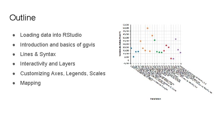
Outline ● Loading data into RStudio ● Introduction and basics of ggvis ● Lines & Syntax ● Interactivity and Layers ● Customizing Axes, Legends, Scales ● Mapping

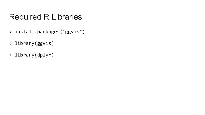
Required R Libraries > install. packages("ggvis") > library(ggvis) > library(dplyr)

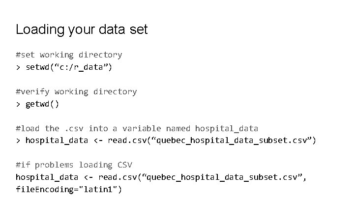
Loading your data set #set working directory > setwd(“c: /r_data”) #verify working directory > getwd() #load the. csv into a variable named hospital_data > hospital_data <- read. csv(“quebec_hospital_data_subset. csv”) #if problems loading CSV hospital_data <- read. csv(“quebec_hospital_data_subset. csv”, file. Encoding="latin 1")

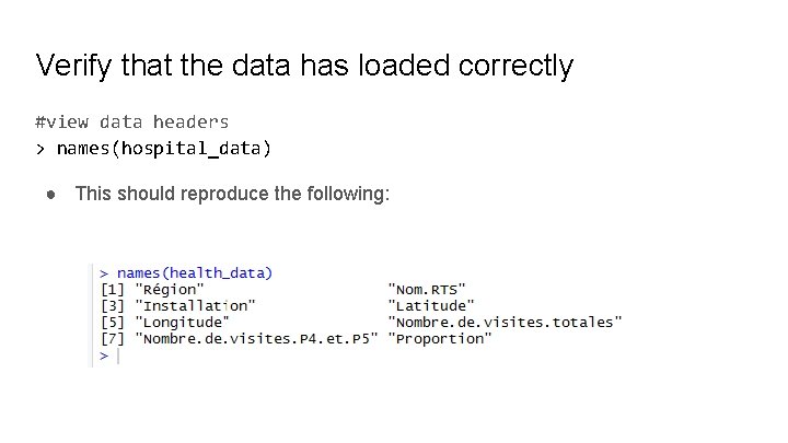
Verify that the data has loaded correctly #view data headers > names(hospital_data) ● This should reproduce the following:

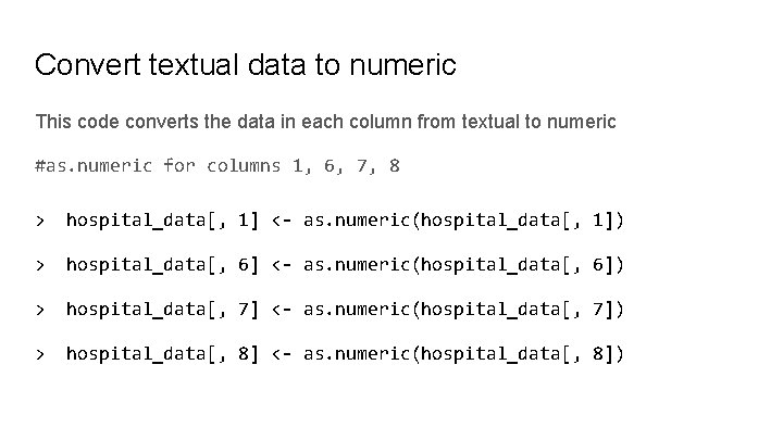
Convert textual data to numeric This code converts the data in each column from textual to numeric #as. numeric for columns 1, 6, 7, 8 > hospital_data[, 1] <- as. numeric(hospital_data[, 1]) > hospital_data[, 6] <- as. numeric(hospital_data[, 6]) > hospital_data[, 7] <- as. numeric(hospital_data[, 7]) > hospital_data[, 8] <- as. numeric(hospital_data[, 8])

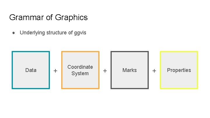
Grammar of Graphics ● Underlying structure of ggvis Data + Coordinate System + Marks + Properties

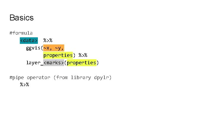
Basics #formula <data> %>% ggvis(~x, ~y, properties) %>% layer_<marks>(properties) #pipe operator (from library dpylr) %>%

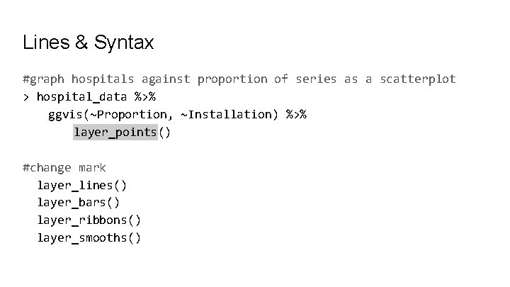
Lines & Syntax #graph hospitals against proportion of series as a scatterplot > hospital_data %>% ggvis(~Proportion, ~Installation) %>% layer_points() #change mark layer_lines() layer_bars() layer_ribbons() layer_smooths()

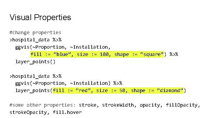
Visual Properties #change properties >hospital_data %>% ggvis(~Proportion, ~Installation, fill : = “blue”, size : = 100, shape : = “square”) %>% layer_points() >hospital_data %>% ggvis(~Proportion, ~Installation) %>% layer_points(fill : = “red”, size : = 50, shape : = “diamond”) #some other properties: stroke, stroke. Width, opacity, fill. Opacity, stroke. Opacity, fill. hover

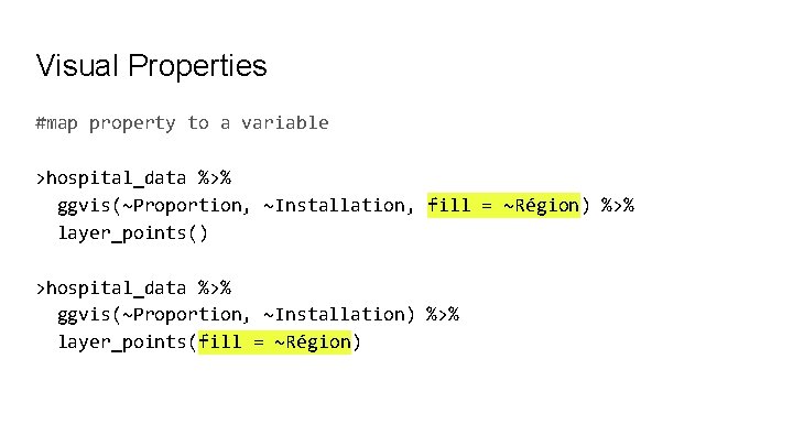
Visual Properties #map property to a variable >hospital_data %>% ggvis(~Proportion, ~Installation, fill = ~Région) %>% layer_points() >hospital_data %>% ggvis(~Proportion, ~Installation) %>% layer_points(fill = ~Région)

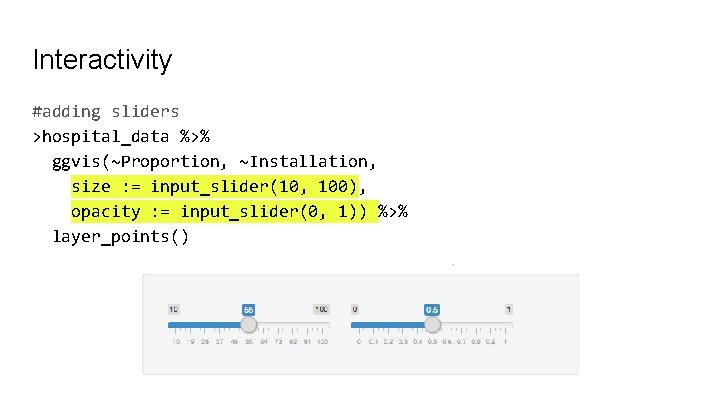
Interactivity #adding sliders >hospital_data %>% ggvis(~Proportion, ~Installation, size : = input_slider(10, 100), opacity : = input_slider(0, 1)) %>% layer_points()

Layers ● Two layer types: simple and compound ● Simple represent basic geometric shapes like lines, points and triangles ● Compound represent data transformations along with one or more simple layers

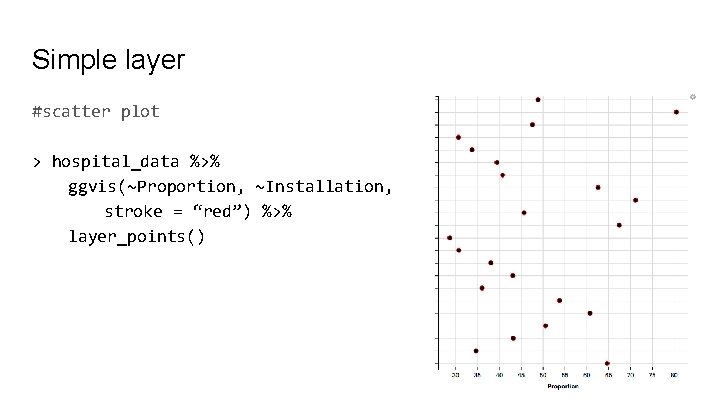
Simple layer #scatter plot > hospital_data %>% ggvis(~Proportion, ~Installation, stroke = “red”) %>% layer_points()

Compound layers ● layer_lines() - order by the x variable ● layer_smooths() - fits a smooth model to the data, and displays predictions in a line

Layer_smooths example #highlights the trend in noisy data > hospital_data %>% ggvis(~Région, ~Nombre. de. visites. totales) %>% layer_smooths() #interactive version > span <- input_slider(1, 5, value=1) hospital_data %>% ggvis(~Région, ~Nombre. de. visites. totales) %>% layer_smooths(span = span)

Customizing axes #create a simple scatter plot and rename x-axis >hospital_data %>% ggvis(~Installation, ~Proportion) %>% layer_points() %>% add_axis("x", title = "Hospital names")

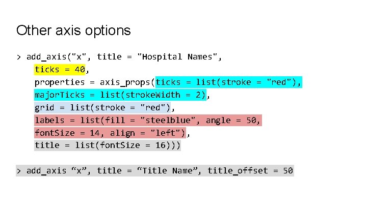
Other axis options > add_axis("x", title = "Hospital Names", ticks = 40, properties = axis_props(ticks = list(stroke = "red"), major. Ticks = list(stroke. Width = 2), grid = list(stroke = "red"), labels = list(fill = "steelblue", angle = 50, font. Size = 14, align = "left"), title = list(font. Size = 16))) > add_axis “x”, title = “Title Name”, title_offset = 50

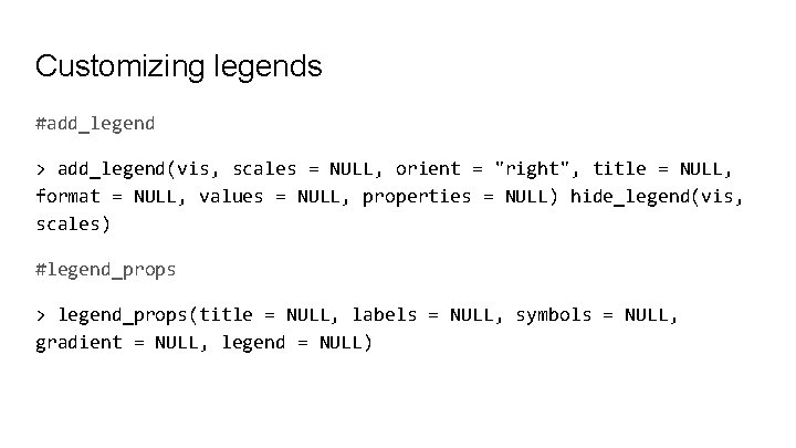
Customizing legends #add_legend > add_legend(vis, scales = NULL, orient = "right", title = NULL, format = NULL, values = NULL, properties = NULL) hide_legend(vis, scales) #legend_props > legend_props(title = NULL, labels = NULL, symbols = NULL, gradient = NULL, legend = NULL)

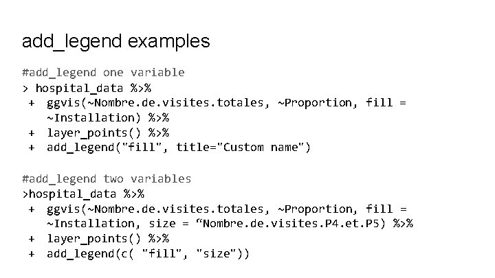
add_legend examples #add_legend one variable > hospital_data %>% + ggvis(~Nombre. de. visites. totales, ~Proportion, fill = ~Installation) %>% + layer_points() %>% + add_legend("fill", title="Custom name") #add_legend two variables >hospital_data %>% + ggvis(~Nombre. de. visites. totales, ~Proportion, fill = ~Installation, size = “Nombre. de. visites. P 4. et. P 5) %>% + layer_points() %>% + add_legend(c( "fill", "size"))

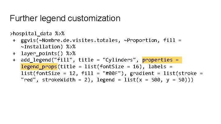
Further legend customization >hospital_data %>% + ggvis(~Nombre. de. visites. totales, ~Proportion, fill = ~Installation) %>% + layer_points() %>% + add_legend("fill", title = "Cylinders", properties = legend_props(title = list(font. Size = 16), labels = list(font. Size = 12, fill = "#00 F"), gradient = list(stroke = "red", stroke. Width = 2), legend = list(x = 500, y = 50)))

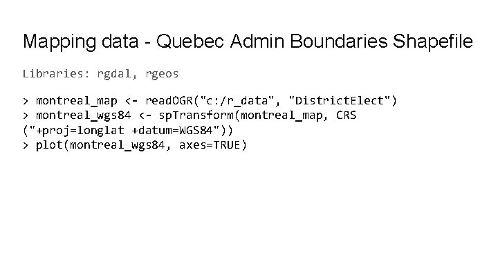
Mapping data - Quebec Admin Boundaries Shapefile Libraries: rgdal, rgeos > montreal_map <- read. OGR("c: /r_data", "District. Elect") > montreal_wgs 84 <- sp. Transform(montreal_map, CRS ("+proj=longlat +datum=WGS 84")) > plot(montreal_wgs 84, axes=TRUE)

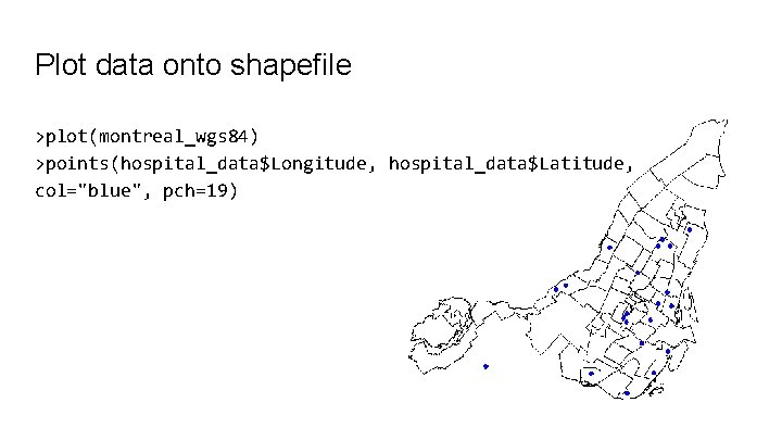
Plot data onto shapefile >plot(montreal_wgs 84) >points(hospital_data$Longitude, hospital_data$Latitude, col="blue", pch=19)

Further documentation ● RStudio ggvis 0. 4 overview ● CPAN documentation