Interactions Interaction Does the relationship between two variables

Interactions • Interaction: Does the relationship between two variables depend on a third variable? – Does the relationship of age to BP depend on gender – Does a certain BP-lowering drug work as well in blacks than in non-blacks – Does the relationship between education and income differ by region of the country Sometimes called “effect modification”

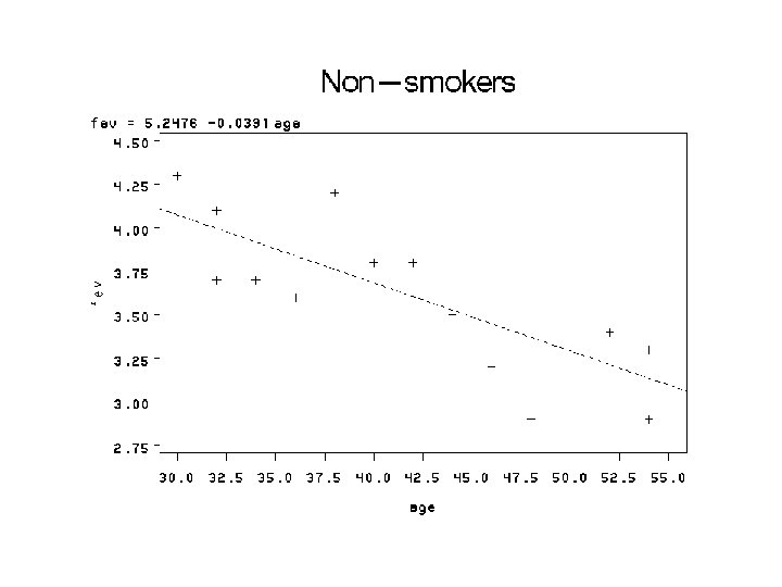
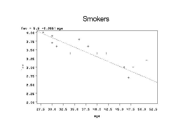
Model for FEV Example Y = b 0 + b 1 X 1 + b 2 X 2 X 1 = smoking status (1=smoker, 0=nonsmoker) X 2 = age Smokers FEV = b 0 + b 1 + b 2 age Non Smokers FEV = b 0 + b 2 age Assumes the slope of age is same for smokers and nonsmokers FEV (smokers) – FEV (non-smokers) = b 1

Non-smokers FEV Smokers b 1 b 2 AGE

Modeling Interaction for FEV Example Y = b 0 + b 1 X 1 + b 2 X 2 + b 3 X 3 X 1 = smoking status (1=smoker, 0=nonsmoker) X 2 = age X 3 = age x smoking status Smokers: FEV = b 0 + b 1 + (b 2 + b 3) age Non Smokers: FEV = b 0 + b 2 age FEV (Smokers) – FEV (Non-smokers) = b 1 + b 3 age Ho: b 3 = 0
")
Non-smokers Note: Difference in slopes implies smoker/nonsmoker difference depends on age (and vice versa) FEV smokers b 1 + b 3 age b 2+ AGE b 3

DATA fev; INFILE DATALINES; INPUT age smk fev; agesmk = age*smk; DATALINES; 28 1 4. 0 30 1 3. 9 30 1 3. 7 31 1 3. 6

PROC REG; MODEL fev = age; PLOT fev*age; WHERE smk=0; TITLE 'Non-smokers'; RUN; PROC REG; MODEL fev = age; PLOT fev*age; WHERE smk=1; TITLE 'Smokers'; RUN;

SMOKERS Variable Intercept age DF Parameter Estimate Standard Error t Value Pr > |t| 1 1 5. 50002 -0. 05508 0. 36163 0. 00885 15. 21 -6. 22 <. 0001 DF Parameter Estimate Standard Error t Value Pr > |t| 1 1 5. 24764 -0. 03911 0. 38050 0. 00887 13. 79 -4. 41 <. 0001 0. 0007 NON SMOKERS Variable Intercept age B 1 for smokers = -0. 05508 B 1 for non-smk = -0. 03911 Are these statistically significant?

PROC REG; MODEL fev = age smk agesmk; RUN; Variable Intercept age smk agesmk DF Parameter Estimate Standard Error t Value Pr > |t| 1 1 5. 24764 -0. 03911 0. 25238 -0. 01597 0. 37846 0. 00882 0. 52482 0. 01253 13. 87 -4. 43 0. 48 -1. 27 <. 0001 0. 0002 0. 6346 0. 2138 Interpretation: B(agesmk) = -0. 01597 is difference in slopes between smk/nonsmk B(age) = -0. 03911 is slope for non-smokers (smk=0) SMOKERS Intercept age 1 1 5. 50002 -0. 05508 0. 36163 0. 00885 15. 21 -6. 22 <. 0001 NON-SMOKERS Intercept age 1 1 5. 24764 -0. 03911 0. 38050 0. 00887 13. 79 -4. 41 <. 0001 0. 0007

Polynomial Regression: Adding Quadratic Term Y = b o + b 1 X + b 2 X 2 • Can be used if linear relationship does not hold – Example: alcohol intake and mortality – Example: cholesterol and mortality • Add a quadratic (squared) term • Can test hypothesis that quadratic term in needed – Ho: b 2 = 0 – Ha: b 2 ≠ 0
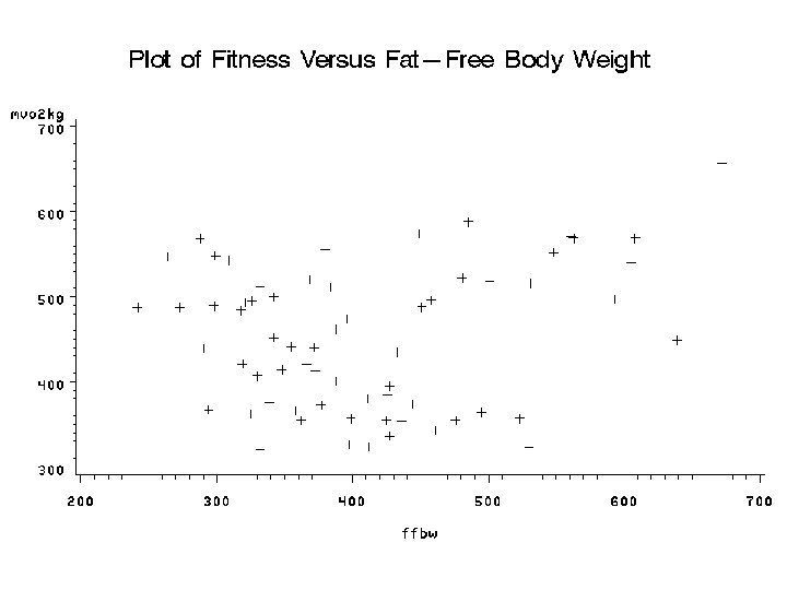

Linear Regression Does not Fit Well

Adding Quadratic Term Plot mvo 2 kg*ffbw predicted. *ffbw/overlay

PROC REG DATA = physfit ; MODEL mvo 2 kg = ffbw; Analysis of Variance Source DF Sum of Squares Model Error Corrected Total 1 69 70 22211 460225 482436 Root MSE Dependent Mean Coeff Variable Intercept ffbw 81. 66965 455. 26761 17. 93882 DF Estimate 1 1 382. 51711 0. 17710 R-Square Adj R-Sq SE 41. 02856 0. 09705 Mean Square 22211 6669. 93228 F Value Pr > F 3. 33 0. 0724 0. 0460 0. 0322 t Value Pr > |t| 9. 32 1. 82 <. 0001 0. 0724

PROC REG DATA = physfit ; ffbw 2 = ffbw * ffbw MODEL mvo 2 kg = ffbw; MODEL mvo 2 kg = ffbw 2; Computed in datastep Analysis of Variance Source DF Sum of Squares Model Error Corrected Total 2 68 70 113179 369257 482436 Root MSE Dependent Mean Coeff Var 73. 69026 455. 26761 16. 18614 R-Square Adj R-Sq Mean Square 56589 5430. 25411 F Value Pr > F 10. 42 0. 0001 0. 2346 0. 2121 Parameter Estimates Variable Intercept ffbw 2 DF Parameter Estimate Standard Error t Value Pr > |t| 1 1 1 980. 95393 -2. 68220 0. 00322 150. 82611 0. 70406 0. 00078761 6. 50 -3. 81 4. 09 <. 0001 0. 0003 0. 0001

Model Selection • Measure many predictors; how do you decide which to include in your model? • Depends on reason for fitting model – Prediction? Examine specific effects? • Statistical criteria do exist, should not be used in place of scientific criteria – Best used in exploratory context

Statistical principles to use • Forward, backward, and stepwise selection – Compare p-values of terms; add/remove based on = 0. 05 or 0. 10 • R 2 methods – Look for models with highest R 2 • Other methods exist

Possible Uses for Using Statistical Criteria • Outcome: Measure of Teenage Drinking – Many Possible Predictors • Questionnaire on relationships, friends, family, church support etc. • Outcome: Echocardographic determined hypertrophy of the heart – Many Possible ECG predictors • Computer measurements from ECG

Backward selection procedure Removes worst variable, then second worst, etc PROC REG DATA = physfit; MODEL mvo 2 kg = male age hgt wgt ffbw rhr / selection=backward; RUN; Final model: Variable Intercept male age wgt ffbw rhr Parameter Estimate 574. 86126 88. 90825 -6. 85862 -6. 00865 0. 75073 -0. 79442 Standard Error Type II SS 56. 50900 12. 02381 3. 80692 1. 02203 0. 12729 0. 41916 167151 88312 5242. 56660 55827 56184 5801. 82822 F Value Pr > F 103. 49 54. 68 3. 25 34. 56 34. 79 3. 59 <. 0001 0. 0762 <. 0001 0. 0625

Forward selection procedure Start with best single variable, adds next best, etc PROC REG DATA = physfit; MODEL mvo 2 kg = male age hgt wgt ffbw rhr / selection=forward; RUN; This example - ends up including all terms except height – Exactly same model as one picked by backward selection

“MAXR” method Select several models based on maximal R 2 PROC REG DATA = physfit; MODEL mvo 2 kg = male age hgt wgt ffbw rhr / selection=maxr; RUN; • Will give “best” models with 1, 2, 3. . . Terms • You choose best overall among the “best”

Final models by MAXR method

Two general principles to use • Parsimony - less is more • Common sense – Don’t use social security number to predict height! • Cautionary Note – Models with several variables are not as good at predicting as model might suggest.
- Slides: 25