Interacting a dummy variable with a continuous variable

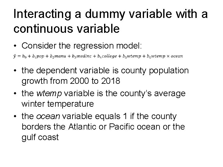
Interacting a dummy variable with a continuous variable • Consider the regression model: • • the dependent variable is county population growth from 2000 to 2018 • the wtemp variable is the county’s average winter temperature • the ocean variable equals 1 if the county borders the Atlantic or Pacific ocean or the gulf coast

Interacting a dummy variable with a continuous variable • • The effect a change in mean winter temperature has on county population growth is given by: • The winter temperature variable (wtemp) shows up twice in the regression model: on its own and interacted (multiplied) with the ocean variable

Interacting a dummy variable with a continuous variable • The marginal effect can be expressed by dividing both sides by the change in wtemp • • The marginal effect winter temperature has on predicted growth can be distinguished between counties that border the ocean (ocean=1) and counties that don’t (ocean=0)

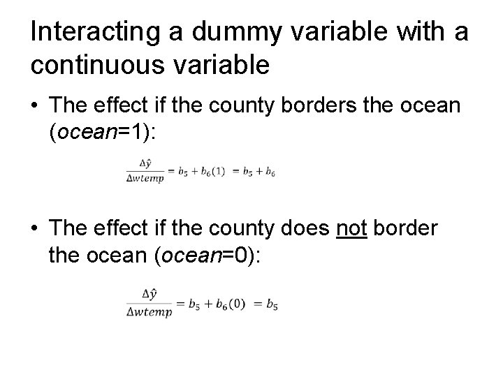
Interacting a dummy variable with a continuous variable • The effect if the county borders the ocean (ocean=1): • The effect if the county does not border the ocean (ocean=0):

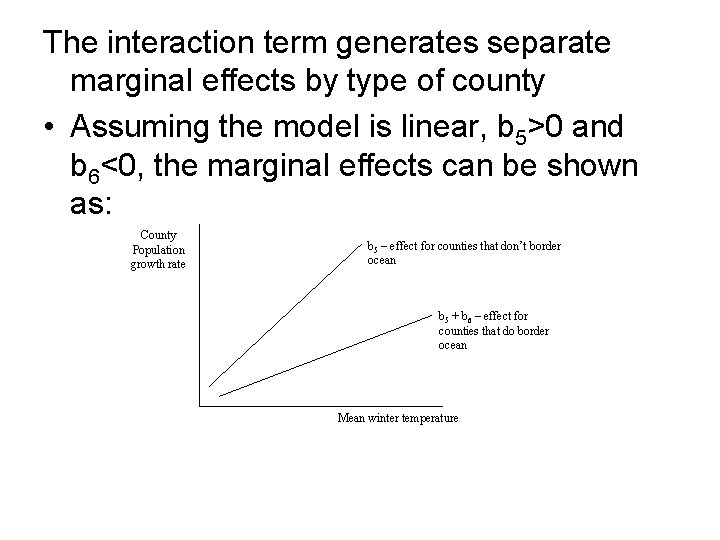
The interaction term generates separate marginal effects by type of county • Assuming the model is linear, b 5>0 and b 6<0, the marginal effects can be shown as: County Population growth rate b 5 – effect for counties that don’t border ocean b 5 + b 6 – effect for counties that do border ocean Mean winter temperature

Hypothesis Tests 1. Test for difference in marginal effect between the two types of counties: H 0: β 6=0 H 1: β 6≠ 0 2. Test for significant effect of mean winter temperature on growth for the counties not bordering the ocean: H 0: β 5=0 H 1: β 5≠ 0

F-test 3. Test for significant effect of mean winter temperature on growth for the counties that border the ocean: H 0: β 5 + β 6 = 0 H 1: β 5 + β 6 ≠ 0 • This hypothesis test follows the F-distribution • The critical value of this test, which is always onetailed, is Fα, q, n-k-1 where α is the level of significance • q represents the number of linear restrictions. In this case one: β 5=-β 6 • n-k-1 is the degrees of freedom in the unrestricted model • In the F-table, the numerator degrees of freedom is q and the denominator degrees of freedom is n-k-1

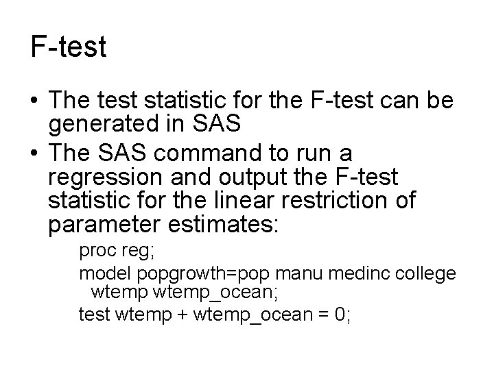
F-test • The test statistic for the F-test can be generated in SAS • The SAS command to run a regression and output the F-test statistic for the linear restriction of parameter estimates: proc reg; model popgrowth=pop manu medinc college wtemp_ocean; test wtemp + wtemp_ocean = 0;