Intensity Transformation Spatial Filtering The term spatial domain

Intensity Transformation & Spatial Filtering The term spatial domain refers to the image plane itself, and methods in that category are based on direct manipulation of pixels in an image. The intensity (or gray-level) transformations & spatial filtering approaches for neighborhood processing, or spatial convolution.

Intensity Transformation & Spatial Filtering Background: The spatial domain processing are denoted by the expression: g(x, y) = T[f(x, y)] where f(x, y) is the input image, g(x, y) is the output (processed) image, and T is an operator on f, defined over a specified neighborhood about point (x, y). In addition, T can be operate on a set of images, such as performing the addition of K images for noise reduction.

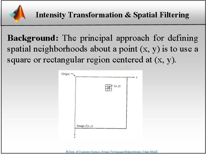
Intensity Transformation & Spatial Filtering Background: The principal approach for defining spatial neighborhoods about a point (x, y) is to use a square or rectangular region centered at (x, y).

Intensity Transformation & Spatial Filtering The center of the pixel is moved from pixel to pixel starting, say , at the top, left, corner, and, it moves, it encompasses different neighborhoods. Operator T is applied at each location (x, y) to yield the output, g, at that location. Only the pixels in the neighborhood computing the values of g at (x, y).

Intensity Transformation & Spatial Filtering Intensity transformation functions: The simplest form of the function T is when the neighborhood in of size 1 x 1 (a single pixel). In this case, the value of g at (x, y) depends only on the intensity of f at that point, and T becomes an intensity or gray level transformation function. When dealing with color images, the term intensity is used to denote a color image component in certain color spaces.

Intensity Transformation & Spatial Filtering Intensity transformation functions: The color images are only depends on intensity values, and not explicitly on (x, y), intensity transformation functions are frequently written in simplified form as: s = T(r) where r denotes the intensity of f and s the intensity of g, both at any corresponding point (x, y) in the images.

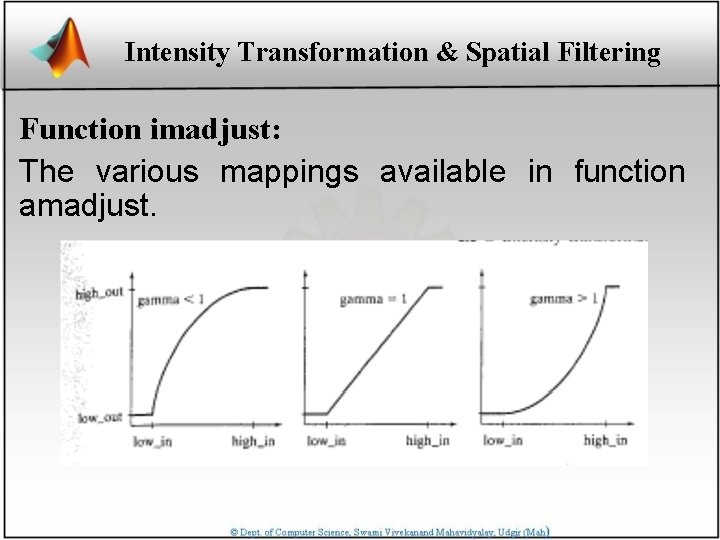
Intensity Transformation & Spatial Filtering Function imadjust: Function imadjust is the basic IPT tool for intensity transformations of gray scale images, it has the following syntax: g= imadjust(f, [low_in high_in, low_out high_out], gamma) This function maps the intensity values in image f to new values in g, such that values between low_in and high_in map to values between low_out and high_out.

Intensity Transformation & Spatial Filtering Function imadjust: The parameter gamma specifies the shape of the curve that maps the intensity values in f to create g. If gamma is less than 1, tha mapping is weighted towards higher (brighter) output values. If gamma greater than 1, the mapping is weighted towards lower (darker) output values. If it is omitted from the function argument, gamma defaults to 1.

Intensity Transformation & Spatial Filtering Function imadjust: The various mappings available in function amadjust.

Intensity Transformation & Spatial Filtering Function imadjust: g 1 = imadjust (f, [0 1], [1 0]); This process is the digital equivalent of obtaining a photographic negative, is particularly useful for enhancing white or gray detail embedded in a large predominantly dark region.

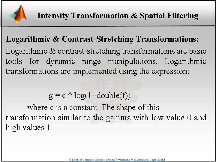
Intensity Transformation & Spatial Filtering Logarithmic & Contrast-Stretching Transformations: Logarithmic & contrast-stretching transformations are basic tools for dynamic range manipulations. Logarithmic transformations are implemented using the expression: g = c * log(1+double(f)) where c is a constant. The shape of this transformation similar to the gamma with low value 0 and high values 1.

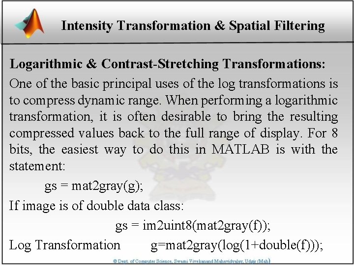
Intensity Transformation & Spatial Filtering Logarithmic & Contrast-Stretching Transformations: One of the basic principal uses of the log transformations is to compress dynamic range. When performing a logarithmic transformation, it is often desirable to bring the resulting compressed values back to the full range of display. For 8 bits, the easiest way to do this in MATLAB is with the statement: gs = mat 2 gray(g); If image is of double data class: gs = im 2 uint 8(mat 2 gray(f)); Log Transformation g=mat 2 gray(log(1+double(f)));

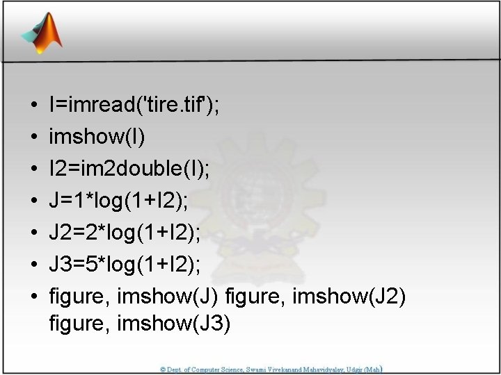
• • I=imread('tire. tif'); imshow(I) I 2=im 2 double(I); J=1*log(1+I 2); J 2=2*log(1+I 2); J 3=5*log(1+I 2); figure, imshow(J) figure, imshow(J 2) figure, imshow(J 3)

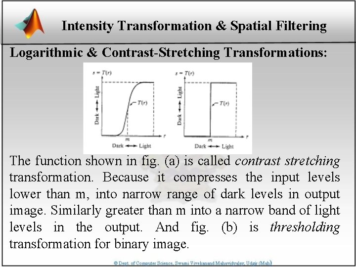
Intensity Transformation & Spatial Filtering Logarithmic & Contrast-Stretching Transformations: The function shown in fig. (a) is called contrast stretching transformation. Because it compresses the input levels lower than m, into narrow range of dark levels in output image. Similarly greater than m into a narrow band of light levels in the output. And fig. (b) is thresholding transformation for binary image.

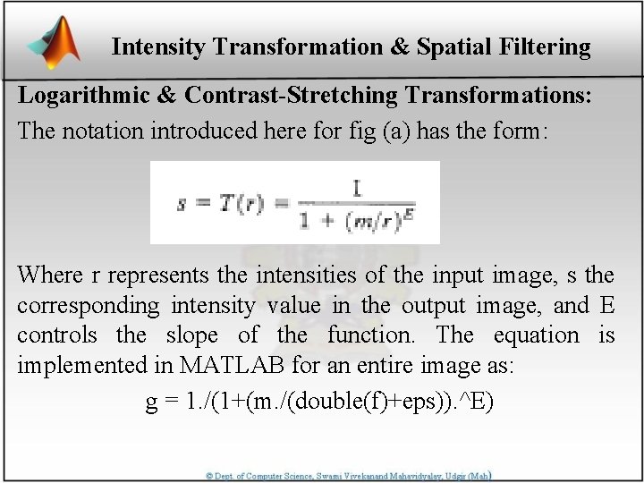
Intensity Transformation & Spatial Filtering Logarithmic & Contrast-Stretching Transformations: The notation introduced here for fig (a) has the form: Where r represents the intensities of the input image, s the corresponding intensity value in the output image, and E controls the slope of the function. The equation is implemented in MATLAB for an entire image as: g = 1. /(1+(m. /(double(f)+eps)). ^E)

• I=imread('tire. tif'); I 2=im 2 double(I); m=mean 2(I 2) contrast 1=1. /(1+(m. /(I 2+eps)). ^4); contrast 2=1. /(1+(m. /(I 2+eps)). ^5); contrast 3=1. /(1+(m. /(I 2+eps)). ^10); imshow(I 2) figure, imshow(contrast 1) figure, imshow(contrast 2) figure, imshow(contrast 3)

Intensity Transformation & Spatial Filtering Histogram Processing & Function Plotting: Intensity transformation function based on information extracted from image intensity histogram play the basic role in image processing, in area such as enhancement, compression, segmentation, and description. Now the focus is on obtaining, plotting, and using histograms for image enhancement.

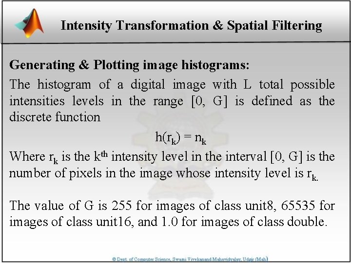
Intensity Transformation & Spatial Filtering Generating & Plotting image histograms: The histogram of a digital image with L total possible intensities levels in the range [0, G] is defined as the discrete function h(rk) = nk Where rk is the kth intensity level in the interval [0, G] is the number of pixels in the image whose intensity level is rk. The value of G is 255 for images of class unit 8, 65535 for images of class unit 16, and 1. 0 for images of class double.

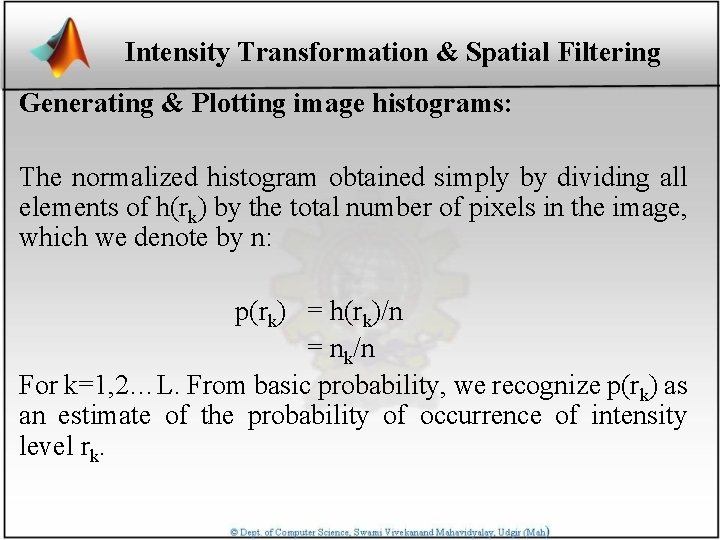
Intensity Transformation & Spatial Filtering Generating & Plotting image histograms: The normalized histogram obtained simply by dividing all elements of h(rk) by the total number of pixels in the image, which we denote by n: p(rk) = h(rk)/n = nk/n For k=1, 2…L. From basic probability, we recognize p(rk) as an estimate of the probability of occurrence of intensity level rk.

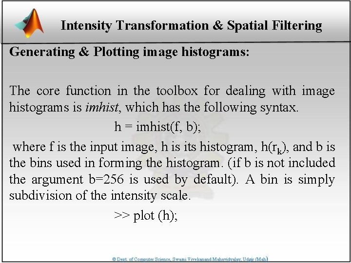
Intensity Transformation & Spatial Filtering Generating & Plotting image histograms: The core function in the toolbox for dealing with image histograms is imhist, which has the following syntax. h = imhist(f, b); where f is the input image, h is its histogram, h(rk), and b is the bins used in forming the histogram. (if b is not included the argument b=256 is used by default). A bin is simply subdivision of the intensity scale. >> plot (h);

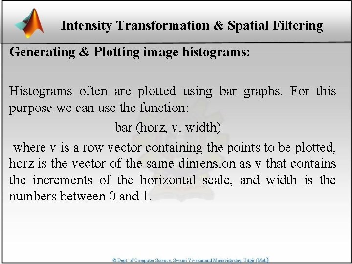
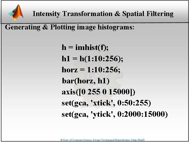
Intensity Transformation & Spatial Filtering Generating & Plotting image histograms: Histograms often are plotted using bar graphs. For this purpose we can use the function: bar (horz, v, width) where v is a row vector containing the points to be plotted, horz is the vector of the same dimension as v that contains the increments of the horizontal scale, and width is the numbers between 0 and 1.

Intensity Transformation & Spatial Filtering Generating & Plotting image histograms: The image histograms can be plot in various ways like a) imhist b) bar c) stem d) plot

Intensity Transformation & Spatial Filtering Generating & Plotting image histograms: h = imhist(f); h 1 = h(1: 10: 256); horz = 1: 10: 256; bar(horz, h 1) axis([0 255 0 15000]) set(gca, 'xtick', 0: 50: 255) set(gca, 'ytick', 0: 2000: 15000)

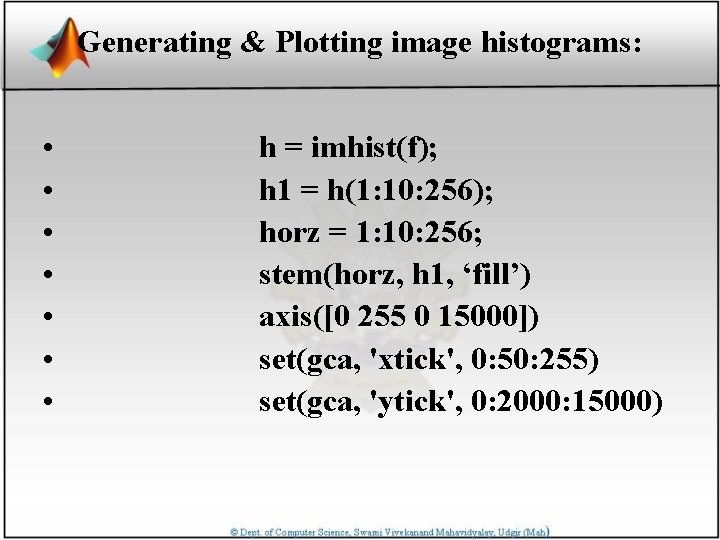
Generating & Plotting image histograms: • • h = imhist(f); h 1 = h(1: 10: 256); horz = 1: 10: 256; stem(horz, h 1, ‘fill’) axis([0 255 0 15000]) set(gca, 'xtick', 0: 50: 255) set(gca, 'ytick', 0: 2000: 15000)

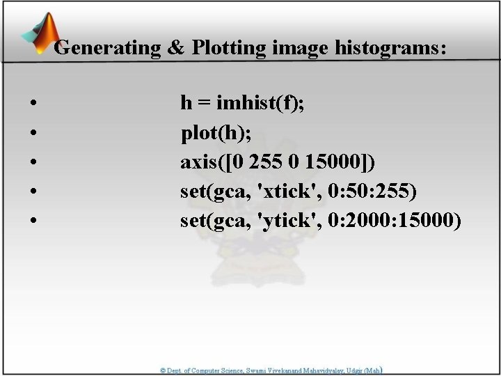
Generating & Plotting image histograms: • • • h = imhist(f); plot(h); axis([0 255 0 15000]) set(gca, 'xtick', 0: 50: 255) set(gca, 'ytick', 0: 2000: 15000)

Intensity Transformation & Spatial Filtering Histogram equalization: f=imread(‘pout. tif’); imshow(f); figure, imhist(f); ylim(‘auto’) g=histeq(f, 256); figure, imshow(g); figure, imhist(g); ylim(‘auto’)

Intensity Transformation & Spatial Filtering: The neighborhood processing consists of 1) Defining a centre point (x, y) 2) Performing an operation on only that pixels in a predefined neighborhood. 3) Letting the result of that operation be the “response” of that process. 4) Repeating the process for every point in the image. The two principal process used to identify this operation are neighborhood processing and spatial filtering.

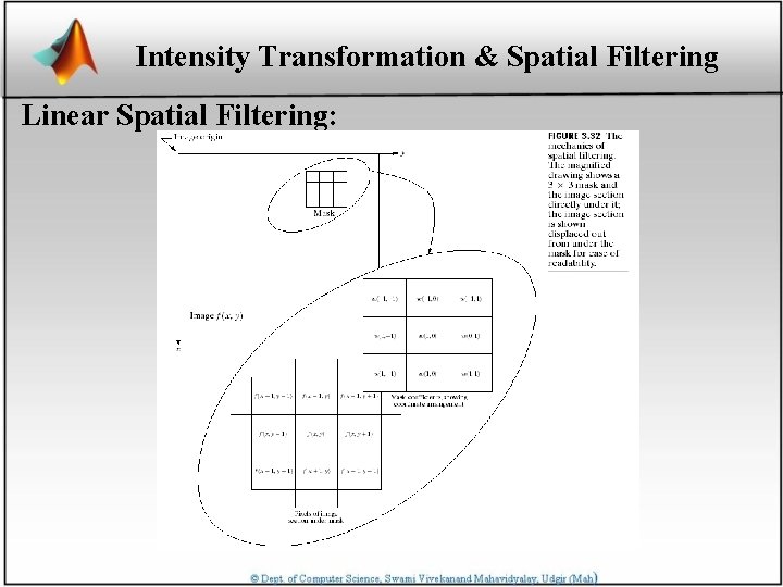
Intensity Transformation & Spatial Filtering Linear Spatial Filtering: The processes consists of moving the centre of the filter mask w from point to point in an image, f. At each point (x, y), the response of the filter at that point is the sum of products of the filter coefficients and the corresponding neighborhood pixels in area. For a mask of size m x n we assume typically that m=2 a+1 n=2 b+1 where a and b are non negative integers.

Intensity Transformation & Spatial Filtering Linear Spatial Filtering:

Intensity Transformation & Spatial Filtering Linear Spatial Filtering: Correlation: is the process of passing the mask w by the image array f through linear neighborhood processing Convolution: is the same process, except that w is rotated by 180 o prior to passing it by f.

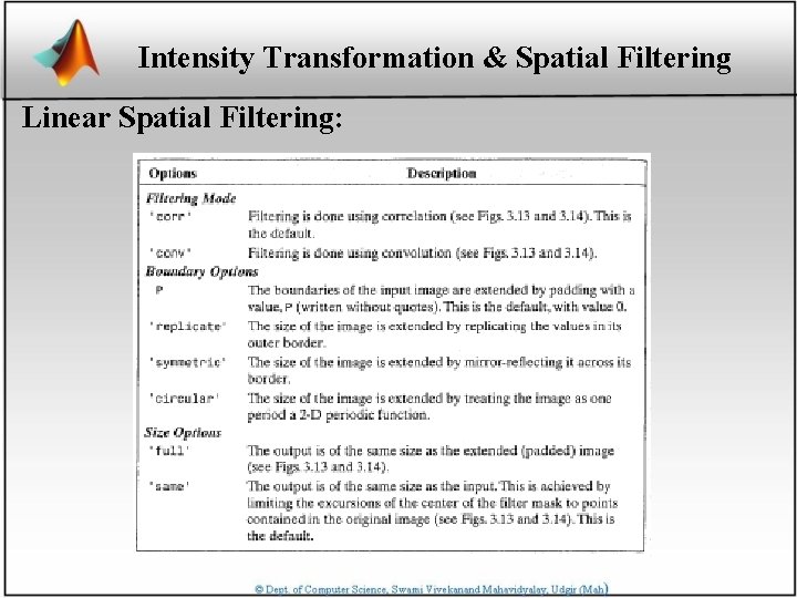
Intensity Transformation & Spatial Filtering Linear Spatial Filtering: The toolbox implements linear spatial filtering using function imfilter which has the following syntax. imfilter(f, w, filtering_mode, boundary_options, size_options) where f is the input image, w is a filter mask, and other parameters are summarized in the next table.

Intensity Transformation & Spatial Filtering Linear Spatial Filtering:

Intensity Transformation & Spatial Filtering Linear Spatial Filtering: The toolbox supports number of predefined 2 -D linear spatial filters, obtained using function fspecial, which generates a filter mask, w, using the syntax w = fspecial(‘type’, parameters) where ‘type’ specifies the filter type, and parameters further defines the specified filter.

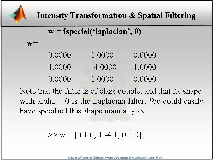
Intensity Transformation & Spatial Filtering w = fspecial(‘laplacian’, 0) w= 0. 0000 1. 0000 -4. 0000 1. 0000 0. 0000 Note that the filter is of class double, and that its shape with alpha = 0 is the Laplacian filter. We could easily have specified this shape manually as >> w = [0 1 0; 1 -4 1; 0 1 0];

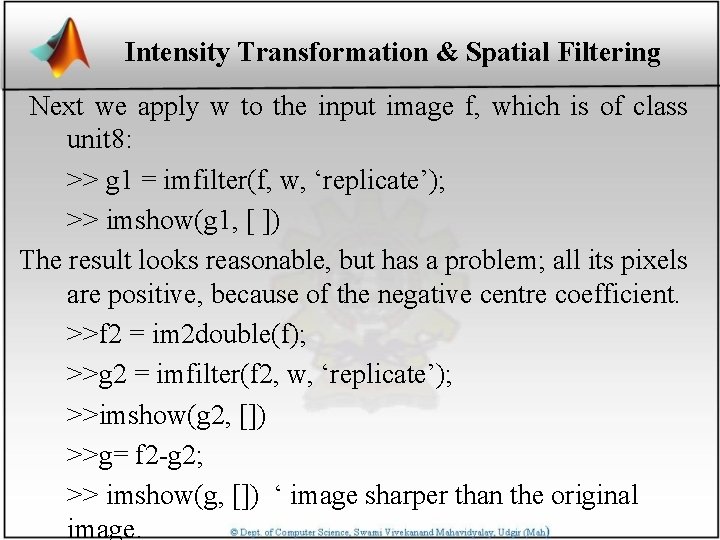
Intensity Transformation & Spatial Filtering Next we apply w to the input image f, which is of class unit 8: >> g 1 = imfilter(f, w, ‘replicate’); >> imshow(g 1, [ ]) The result looks reasonable, but has a problem; all its pixels are positive, because of the negative centre coefficient. >>f 2 = im 2 double(f); >>g 2 = imfilter(f 2, w, ‘replicate’); >>imshow(g 2, []) >>g= f 2 -g 2; >> imshow(g, []) ‘ image sharper than the original image.

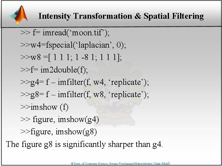
Intensity Transformation & Spatial Filtering >> f= imread(‘moon. tif’); >>w 4=fspecial(‘laplacian’, 0); >>w 8 =[ 1 1 1; 1 -8 1; 1 1 1]; >>f= im 2 double(f); >>g 4= f – imfilter(f, w 4, ‘replicate’); >>g 8= f – imfilter(f, w 8, ‘replicate’); >>imshow (f) >> figure, imshow(g 4) >>figure, imshow(g 8) The figure g 8 is significantly sharper than g 4.