Intelligent Systems AI2 Computer Science cpsc 422 Lecture

Intelligent Systems (AI-2) Computer Science cpsc 422, Lecture 12 Sept, 30, 2019 Slide credit: some slides adapted from Stuart Russell (Berkeley) CPSC 422, Lecture 12 Slide 1

Lecture Overview • Recap of Forward and Rejection Sampling • Likelihood Weighting • Monte Carlo Markov Chain (MCMC) – Gibbs Sampling • Application Requiring Approx. reasoning CPSC 422, Lecture 12 2

Sampling The building block on any sampling algorithm is the generation of samples from a known (or easy to compute, like in Gibbs) distribution We then use these samples to derive estimates of probabilities hard-to-compute exactly And you want consistent sampling methods. . . More samples. . . Closer to. . . CPSC 422, Lecture 12 Slide 3

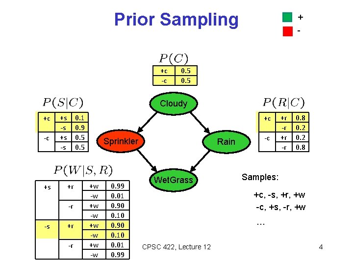
Prior Sampling +c -c + - 0. 5 Cloudy +c -c +s +s -s 0. 1 0. 9 0. 5 +r -r -s +r -r +c Sprinkler +w -w 0. 99 0. 01 0. 90 0. 10 0. 01 0. 99 Rain Wet. Grass -c +r -r 0. 8 0. 2 0. 8 Samples: +c, -s, +r, +w -c, +s, -r, +w … CPSC 422, Lecture 12 4

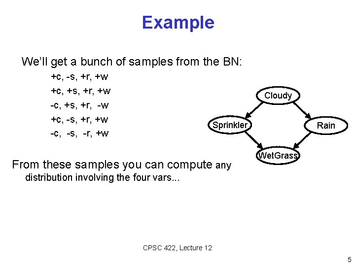
Example We’ll get a bunch of samples from the BN: +c, -s, +r, +w +c, +s, +r, +w -c, +s, +r, -w +c, -s, +r, +w -c, -s, -r, +w Cloudy Sprinkler From these samples you can compute any Rain Wet. Grass distribution involving the four vars. . . CPSC 422, Lecture 12 5

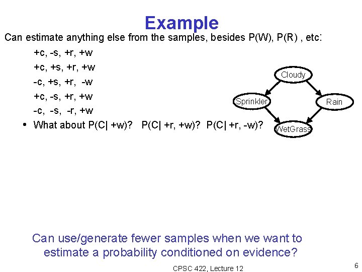
Example Can estimate anything else from the samples, besides P(W), P(R) , etc: +c, -s, +r, +w +c, +s, +r, +w Cloudy -c, +s, +r, -w +c, -s, +r, +w Sprinkler -c, -s, -r, +w • What about P(C| +w)? P(C| +r, -w)? Wet. Grass Rain Can use/generate fewer samples when we want to estimate a probability conditioned on evidence? CPSC 422, Lecture 12 6

Rejection Sampling Let’s say we want P(W| +s) • ignore (reject) samples which don’t • • C S have S=+s This is called rejection sampling It is also consistent for conditional probabilities (i. e. , correct in the limit) But what happens if +s is rare? R W +c, -s, +r, +w +c, +s, +r, +w -c, +s, +r, -w +c, -s, +r, +w -c, -s, -r, +w And if the number of evidence vars grows. . . A. Less samples will be rejected B. More samples will be rejected CPSC 422, Lecture 12 C. The same number of samples will be rejected 7

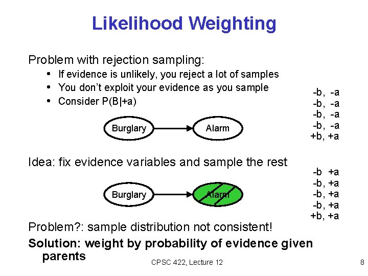
Likelihood Weighting Problem with rejection sampling: • If evidence is unlikely, you reject a lot of samples • You don’t exploit your evidence as you sample • Consider P(B|+a) Burglary Alarm Idea: fix evidence variables and sample the rest Burglary Alarm -b, -a +b, +a -b, +a +b, +a Problem? : sample distribution not consistent! Solution: weight by probability of evidence given parents CPSC 422, Lecture 12 8

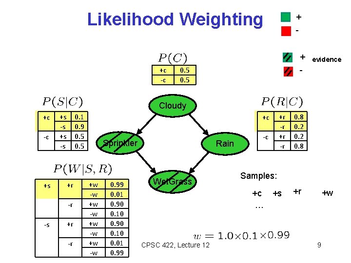
Likelihood Weighting +c -c + + - 0. 5 evidence Cloudy +c -c +s +s -s 0. 1 0. 9 0. 5 +r -r -s +r -r +c Sprinkler +w -w 0. 99 0. 01 0. 90 0. 10 0. 01 0. 99 Rain Wet. Grass -c +r -r Samples: +c +s … CPSC 422, Lecture 12 0. 8 0. 2 0. 8 +r +w 9

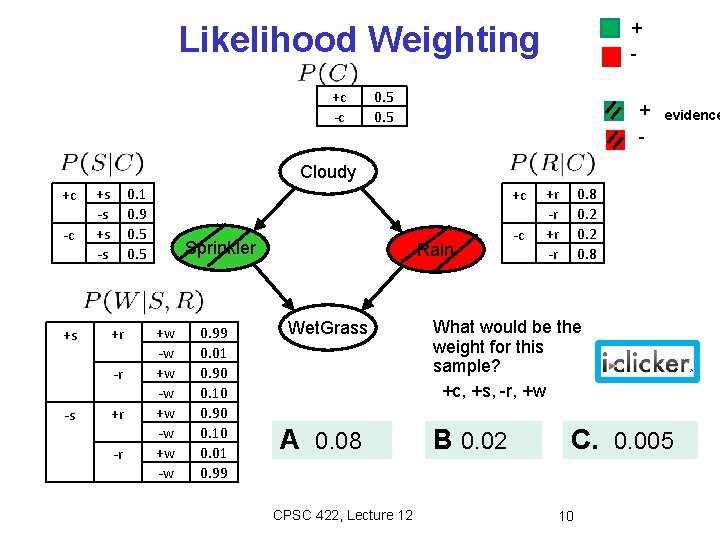
+ - Likelihood Weighting +c -c 0. 5 + - evidence Cloudy +c -c +s +s -s 0. 1 0. 9 0. 5 +r -r -s +r -r +c Sprinkler +w -w 0. 99 0. 01 0. 90 0. 10 0. 01 0. 99 Rain Wet. Grass A 0. 08 CPSC 422, Lecture 12 -c +r -r 0. 8 0. 2 0. 8 What would be the weight for this sample? +c, +s, -r, +w B 0. 02 C. 0. 005 10

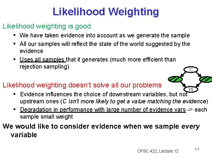
Likelihood Weighting Likelihood weighting is good • We have taken evidence into account as we generate the sample • All our samples will reflect the state of the world suggested by the • evidence Uses all samples that it generates (much more efficient than rejection sampling) Cloudy C S Likelihood weighting doesn’t solve all our problems W • Evidence influences the choice of downstream variables, but not • Rain R upstream ones (C isn’t more likely to get a value matching the evidence) Degradation in performance with large number of evidence vars -> each sample small weight We would like to consider evidence when we sample every variable CPSC 422, Lecture 12 11

Lecture Overview • Recap of Forward and Rejection Sampling • Likelihood Weighting • Monte Carlo Markov Chain (MCMC) – Gibbs Sampling • Application Requiring Approx. reasoning CPSC 422, Lecture 12 12

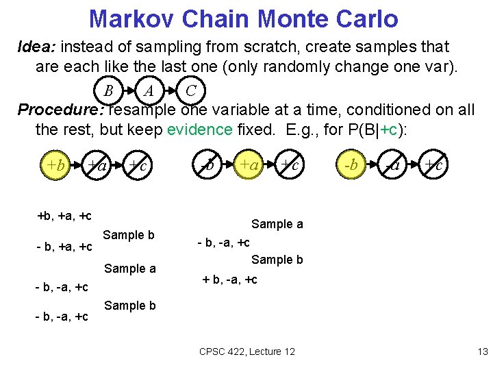
Markov Chain Monte Carlo Idea: instead of sampling from scratch, create samples that are each like the last one (only randomly change one var). B A C Procedure: resample one variable at a time, conditioned on all the rest, but keep evidence fixed. E. g. , for P(B|+c): +b +a +c -b +a +b, +a, +c - b, +a, +c Sample b Sample a - b, -a, +c +c -b -a +c Sample a - b, -a, +c Sample b + b, -a, +c Sample b CPSC 422, Lecture 12 13

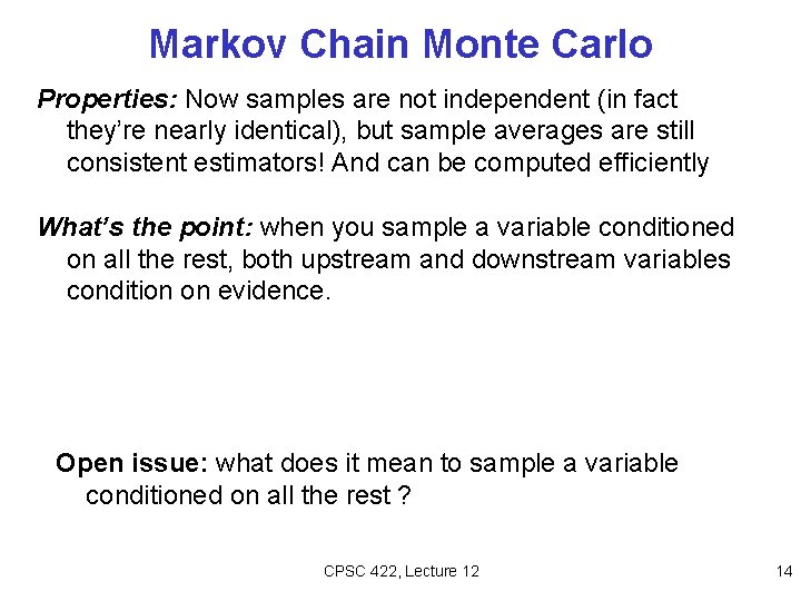
Markov Chain Monte Carlo Properties: Now samples are not independent (in fact they’re nearly identical), but sample averages are still consistent estimators! And can be computed efficiently What’s the point: when you sample a variable conditioned on all the rest, both upstream and downstream variables condition on evidence. Open issue: what does it mean to sample a variable conditioned on all the rest ? CPSC 422, Lecture 12 14

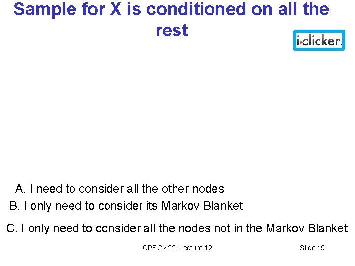
Sample for X is conditioned on all the rest A. I need to consider all the other nodes B. I only need to consider its Markov Blanket C. I only need to consider all the nodes not in the Markov Blanket CPSC 422, Lecture 12 Slide 15

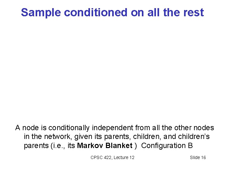
Sample conditioned on all the rest A node is conditionally independent from all the other nodes in the network, given its parents, children, and children’s parents (i. e. , its Markov Blanket ) Configuration B CPSC 422, Lecture 12 Slide 16

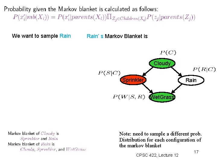
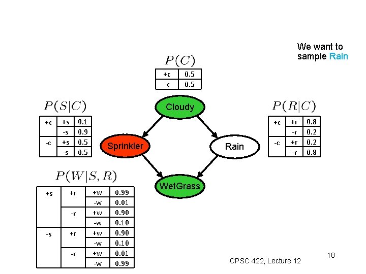
We want to sample Rain’ s Markov Blanket is Cloudy Sprinkler Rain Wet. Grass Note: need to sample a different prob. Distribution for each configuration of the markov blanket CPSC 422, Lecture 12 17

We want to sample Rain +c -c 0. 5 Cloudy +c -c +s +s -s 0. 1 0. 9 0. 5 +r -r -s +r -r +c Sprinkler +w -w 0. 99 0. 01 0. 90 0. 10 0. 01 0. 99 Rain -c +r -r 0. 8 0. 2 0. 8 Wet. Grass CPSC 422, Lecture 12 18

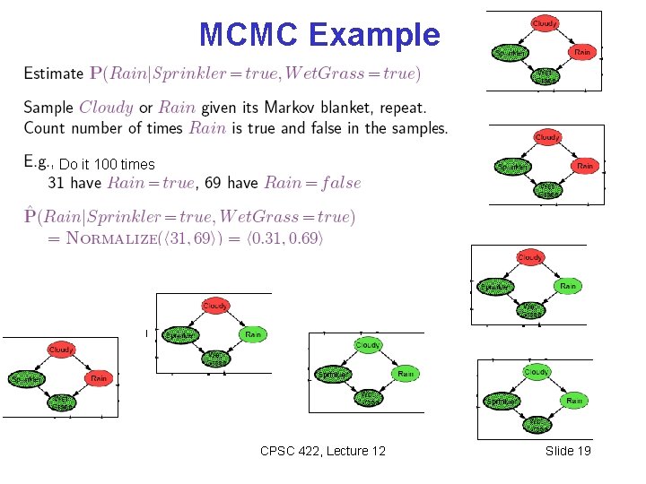
MCMC Example Do it 100 times CPSC 422, Lecture 12 Slide 19

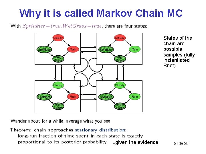
Why it is called Markov Chain MC States of the chain are possible samples (fully instantiated Bnet) . . given the evidence CPSC 422, Lecture 12 Slide 20

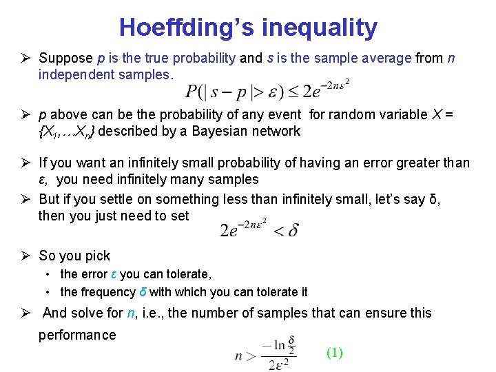
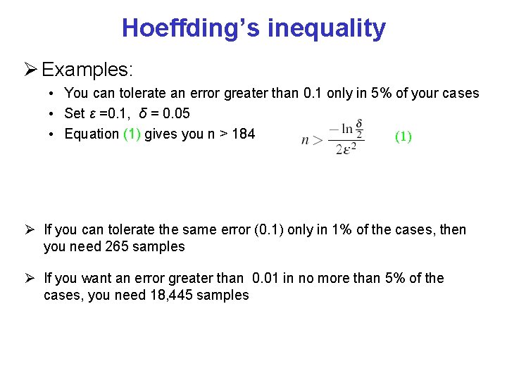
Hoeffding’s inequality Suppose p is the true probability and s is the sample average from n independent samples. p above can be the probability of any event for random variable X = {X 1, …Xn} described by a Bayesian network If you want an infinitely small probability of having an error greater than ε, you need infinitely many samples But if you settle on something less than infinitely small, let’s say δ, then you just need to set So you pick • the error ε you can tolerate, • the frequency δ with which you can tolerate it And solve for n, i. e. , the number of samples that can ensure this performance (1)

Hoeffding’s inequality Examples: • You can tolerate an error greater than 0. 1 only in 5% of your cases • Set ε =0. 1, δ = 0. 05 • Equation (1) gives you n > 184 (1) If you can tolerate the same error (0. 1) only in 1% of the cases, then you need 265 samples If you want an error greater than 0. 01 in no more than 5% of the cases, you need 18, 445 samples

Learning Goals for today’s class You can: • Describe and justify the Likelihood Weighting sampling method • Describe and justify Markov Chain Monte Carlo sampling method CPSC 422, Lecture 12 Slide 23

TODO for Wed Next research paper: Using Bayesian Networks to Manage Uncertainty in Student Modeling. Journal of User Modeling and User-Adapted Interaction 2002 Dynamic BN (required only up to page 400, do not have to answer the question “How was the system evaluated? ) Very influential paper 500+ citations • Follow instructions on course Web. Page <Readings> • Keep working on assignment-2 (due on Fri, Oct 18) CPSC 422, Lecture 12 Slide 24

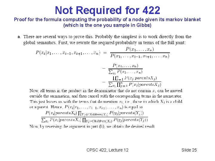
Not Required for 422 Proof for the formula computing the probability of a node given its markov blanket (which is the one you sample in Gibbs) CPSC 422, Lecture 12 Slide 25