Intelligent data analysis Biomarker discovery II Peter Antal

Intelligent data analysis Biomarker discovery II. Peter Antal antal@mit. bme. hu

Overview • Biomarkers • The Bayesian statistical approach • Partial multivariate analysis • Marginalization, sub-, sup-relevance • Frontlines – Causal, confounded extension – Multitarget (multidimensional)extension – Interpretation • Optimal reporting • Fusion: Data analytic knowledge bases • Bayes. Eye

Biomarker challenges in biomedicine • Better outcome variable – „Lost in diagnosis”: phenome • Better and more complete set of predictor variables – „Right under everyone’s noses”: rare variants (RVs) – „The great beyond”: Epigenetics, environment • Better statistical models – „In the architecture”: structural variations – „Out of sight”: many, small effects – „In underground networks”: epistatic interactions • • Causation (confounding) Statistical significance („multiple testing problem”) Complex models: interactions, epistatis Interpretation 3

Causal vs. diagnostic markers Direct =/= Causal SNP-B (“causal”) SNP-A (measured) Mutation Onset Disease Therapic value (e. g. Drug target) Disease Symptoms Diagnostic value Stress Objective (real/causal) diagnostic value? Symptoms

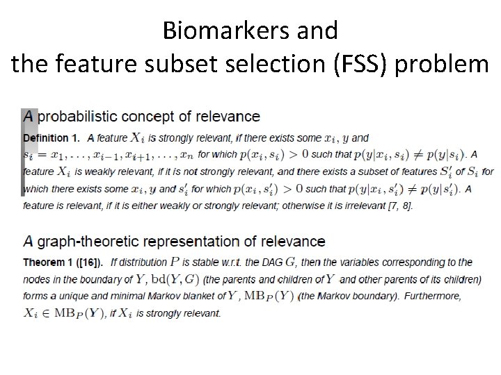
Biomarkers and the feature subset selection (FSS) problem

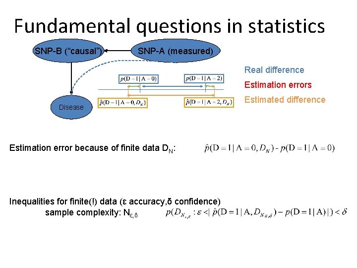
Fundamental questions in statistics SNP-B (“causal”) SNP-A (measured) Real difference Estimation errors Disease Estimation error because of finite data DN: Inequalities for finite(!) data (ε accuracy, δ confidence) sample complexity: Nε, δ Estimated difference

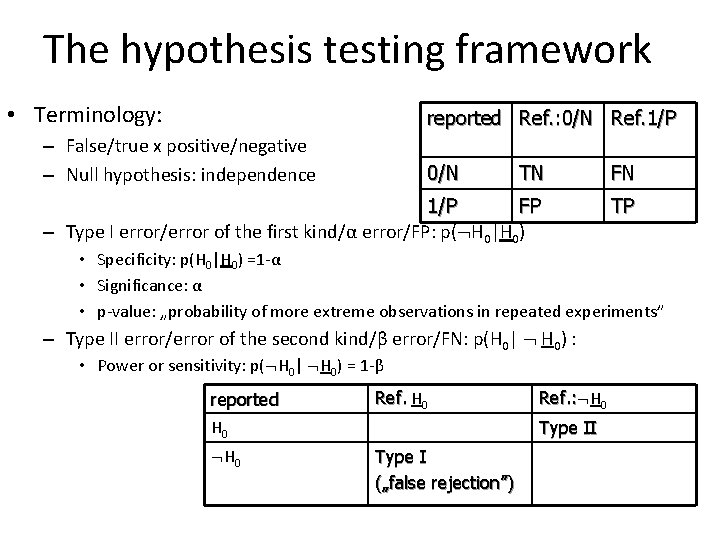
The hypothesis testing framework • Terminology: reported Ref. : 0/N Ref. 1/P – False/true x positive/negative – Null hypothesis: independence 0/N TN FN 1/P FP – Type I error/error of the first kind/α error/FP: p( H 0|H 0) TP • Specificity: p(H 0|H 0) =1 -α • Significance: α • p-value: „probability of more extreme observations in repeated experiments” – Type II error/error of the second kind/β error/FN: p(H 0| H 0) : • Power or sensitivity: p( H 0| H 0) = 1 -β reported H 0 Ref. H 0 Type I („false rejection”) Ref. : H Ref. : 0 Type II

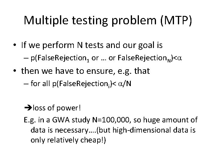
Multiple testing problem (MTP) • If we perform N tests and our goal is – p(False. Rejection 1 or … or False. Rejection. N)<α • then we have to ensure, e. g. that – for all p(False. Rejectioni)< α/N loss of power! E. g. in a GWA study N=100, 000, so huge amount of data is necessary…. (but high-dimensional data is only relatively cheap!)

Solutions for MTP • Corrections • Permutation tests – Generate perturbed data sets under the null hypothesis: permute predictors and outcome. • False discovery rate, q-value • Bayesian approach

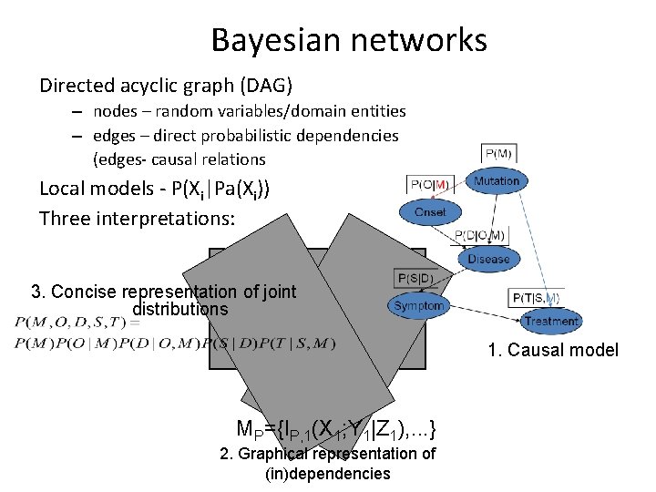
Bayesian networks Directed acyclic graph (DAG) – nodes – random variables/domain entities – edges – direct probabilistic dependencies (edges- causal relations Local models - P(Xi|Pa(Xi)) Three interpretations: 3. Concise representation of joint distributions 1. Causal model MP={IP, 1(X 1; Y 1|Z 1), . . . } 2. Graphical representation of (in)dependencies

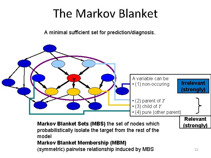
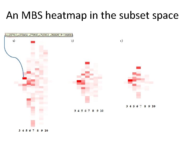
The Markov Blanket A minimal sufficient set for prediction/diagnosis. Y A variable can be: • (1) non-occuring Irrelevant (strongly) • (2) parent of Y • (3) child of Y • (4) pure (other parent) Markov Blanket Sets (MBS) the set of nodes which probabilistically isolate the target from the rest of the model Markov Blanket Membership (MBM) (symmetric) pairwise relationship induced by MBS Relevant (strongly) 11

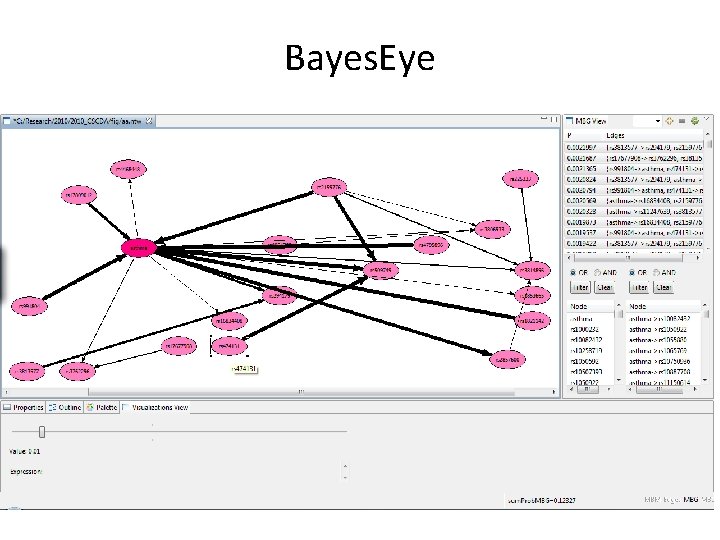
Bayes. Eye

Access to Bayes. Eye • http: //redmine. genagrid. eu – bayeseyestudent – bayes 123 szem • Bayes. Eye. Genagrid – student_${i} – stu${i}dent

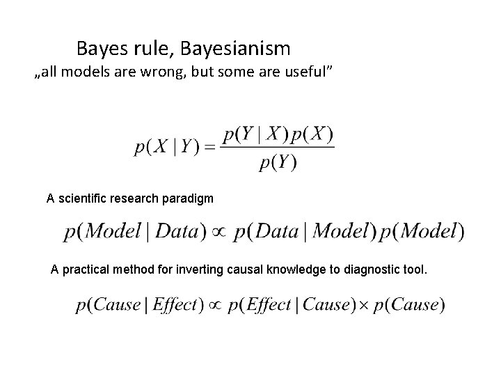
Bayes rule, Bayesianism „all models are wrong, but some are useful” A scientific research paradigm A practical method for inverting causal knowledge to diagnostic tool.

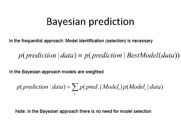
Bayesian prediction In the frequentist approach: Model identification (selection) is necessary In the Bayesian approach models are weighted Note: in the Bayesian approach there is no need for model selection

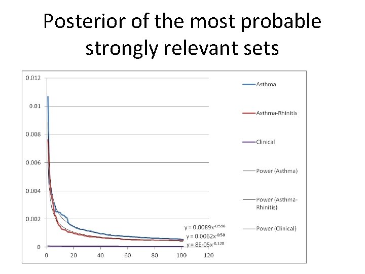
Posterior of the most probable strongly relevant sets

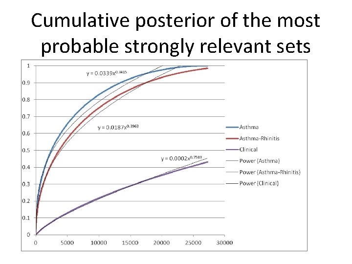
Cumulative posterior of the most probable strongly relevant sets

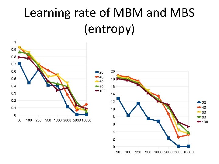
Learning rate of MBM and MBS (entropy)

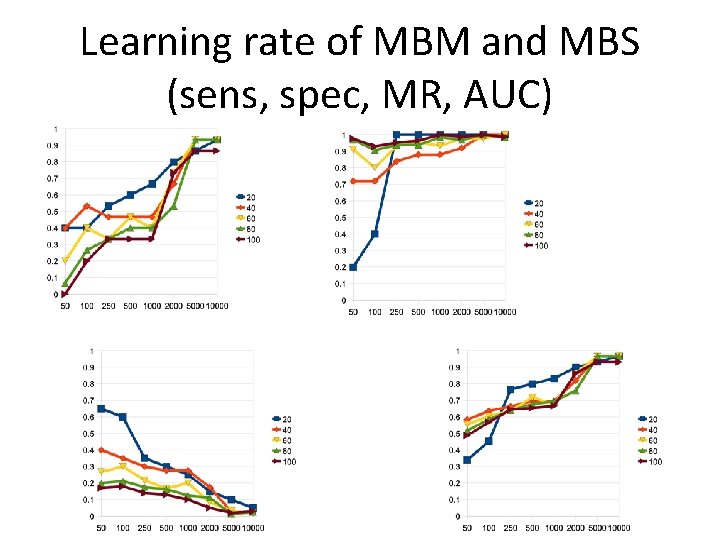
Learning rate of MBM and MBS (sens, spec, MR, AUC)

Frequentist vs Bayesian statistics Frequentist Bayesian - Prior probabilities Null hypothesis - Indirect: proving by refutation Direct Model selection Model averaging Likelihood ratio test Bayes factor p-value -! -! Posterior probabilities Confidence interval Credible region Significance level Optimal decision based on Exp. Util. Multiple testing problem Remains, so complex model Model complexity dilemma Best achievable alternative • Note: direct probabilistic statement!

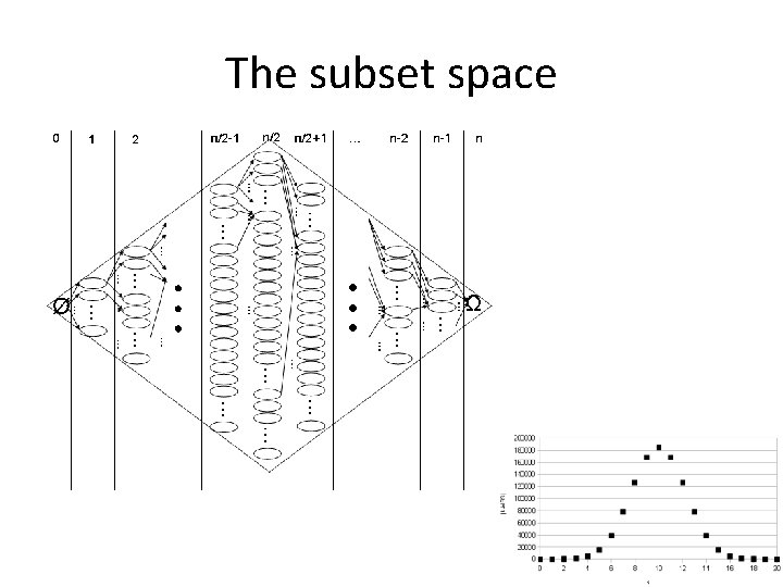
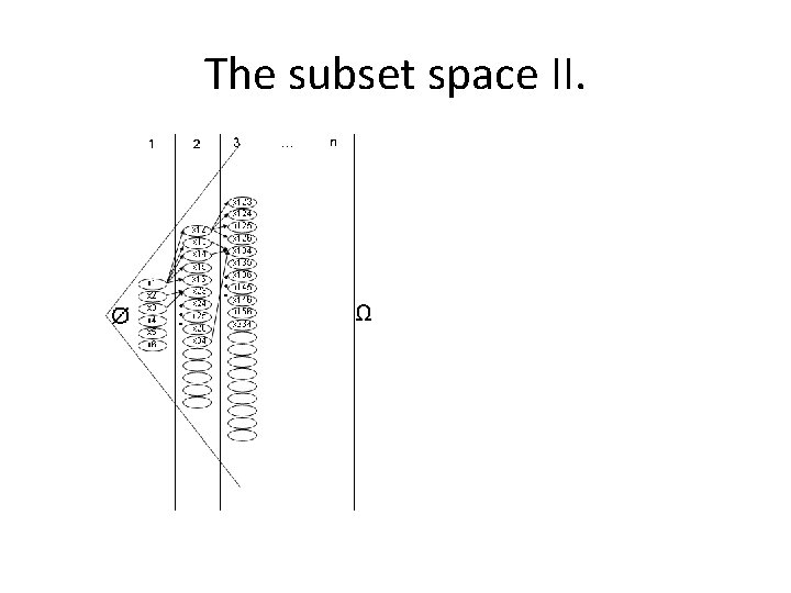
The subset space

The subset space II.

An MBS heatmap in the subset space

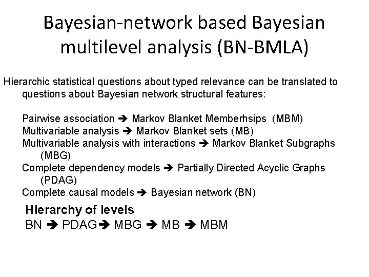
Bayesian-network based Bayesian multilevel analysis (BN-BMLA) Hierarchic statistical questions about typed relevance can be translated to questions about Bayesian network structural features: Pairwise association Markov Blanket Memberhsips (MBM) Multivariable analysis Markov Blanket sets (MB) Multivariable analysis with interactions Markov Blanket Subgraphs (MBG) Complete dependency models Partially Directed Acyclic Graphs (PDAG) Complete causal models Bayesian network (BN) Hierarchy of levels BN PDAG MBG MBM

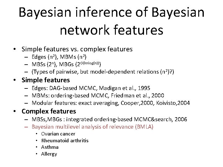
Bayesian inference of Bayesian network features • Simple features vs. complex features – Edges (n 2), MBMs (n 2) – MBSs (2 n), MBGs (2 O(knlog(n))) – (Types of pairwise, but model-dependent relations (n 2)? ) • Simple features – Edges: DAG-based MCMC, Madigan et al. , 1995 – MBMs: ordering-based MCMC, Friedman et al. , 2000 – Modular features: exact averaging, Cooper, 2000, Koivisto, 2004 • Complex features – MBSs, MBGs : integrated ordering-based MCMC&search, 2006 – Bayesian multilevel analysis of relevance (BMLA) • • Ovarian cancer Rheumatoid arthritis Asthma Allergy

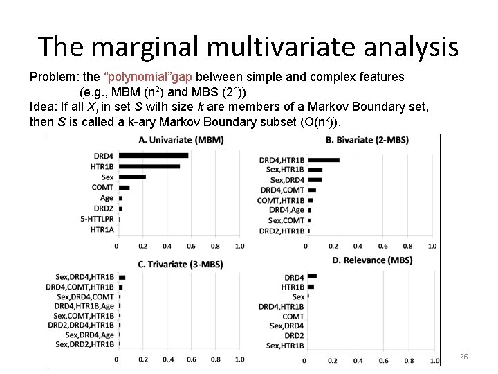
The marginal multivariate analysis Problem: the “polynomial”gap between simple and complex features (e. g. , MBM (n 2) and MBS (2 n)) Idea: If all Xi in set S with size k are members of a Markov Boundary set, then S is called a k-ary Markov Boundary subset (O(nk)). 26

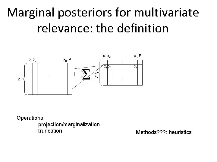
Marginal posteriors for multivariate relevance: the definition Operations: projection/marginalization truncation Methods? ? ? : heuristics

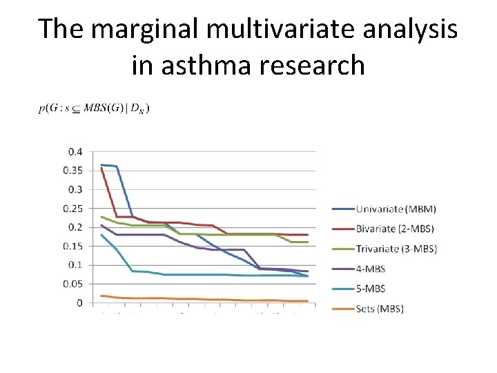
The marginal multivariate analysis in asthma research

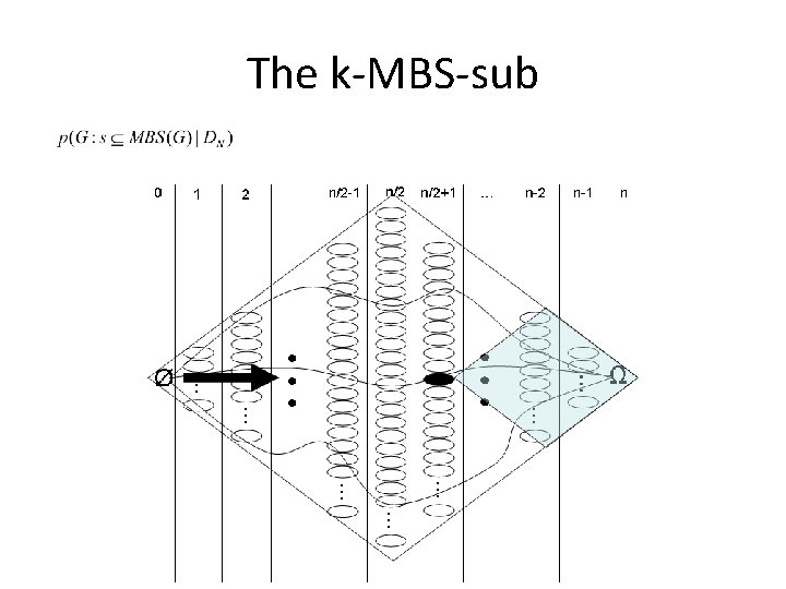
The k-MBS-sub

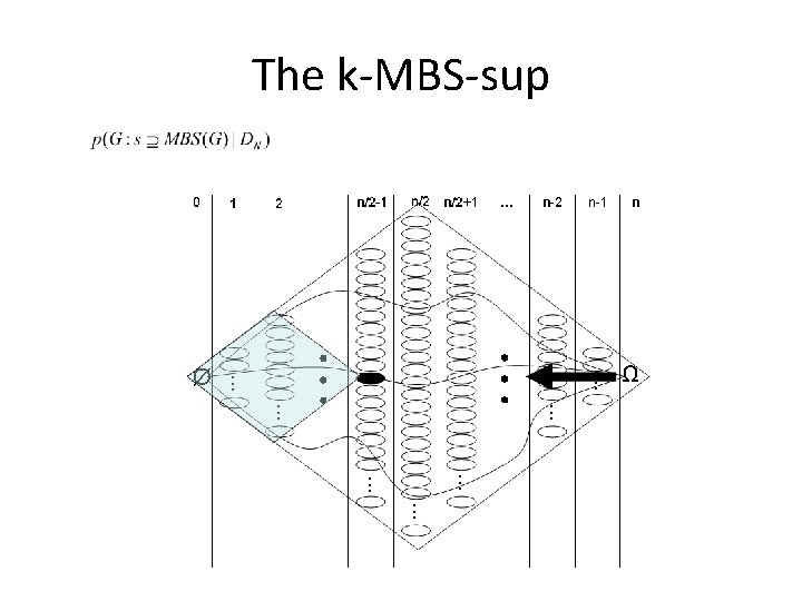
The k-MBS-sup

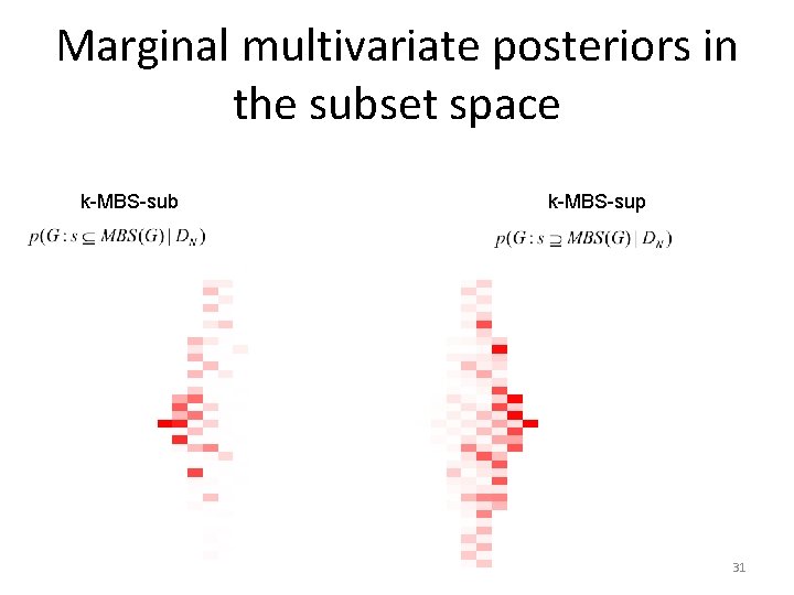
Marginal multivariate posteriors in the subset space k-MBS-sub k-MBS-sup 31

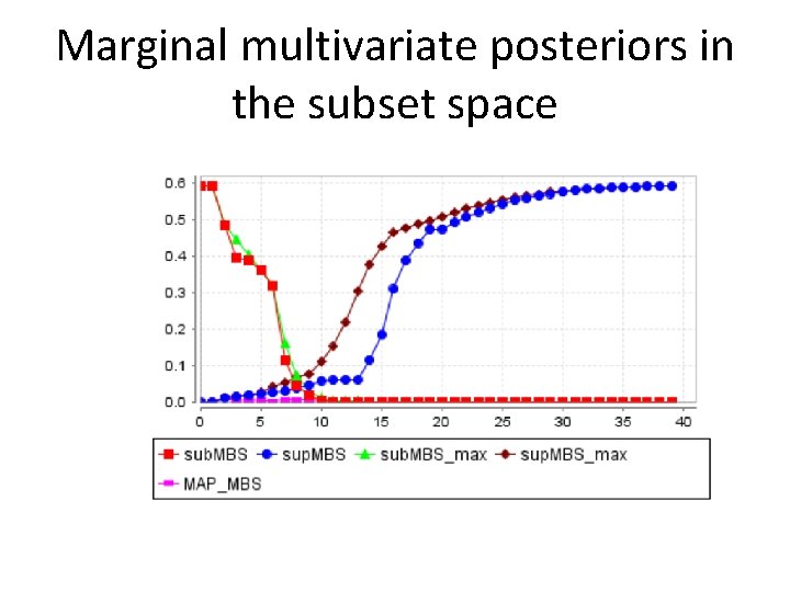
Marginal multivariate posteriors in the subset space

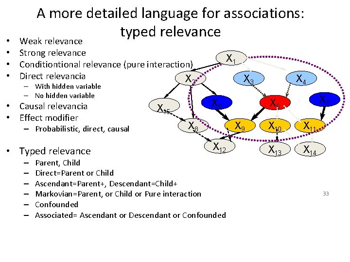
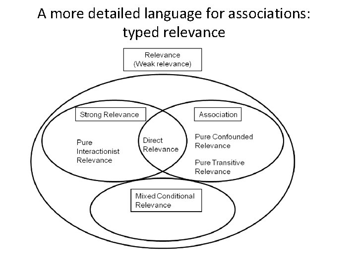
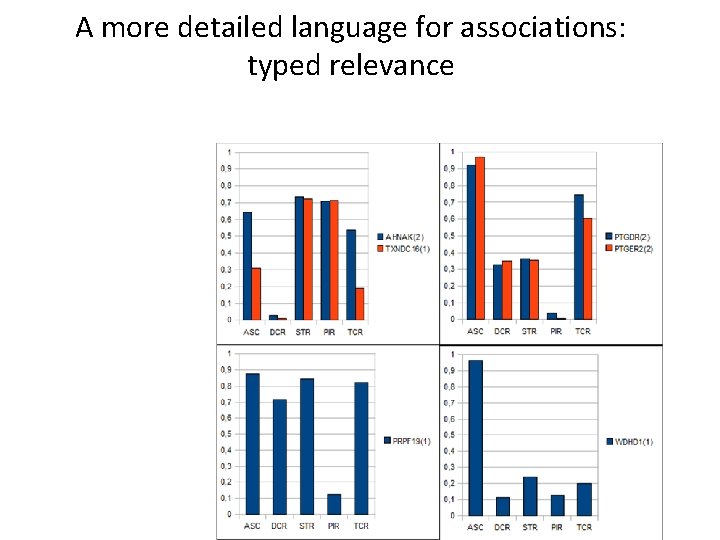
A more detailed language for associations: typed relevance Weak relevance • • Strong relevance • Conditional relevance (pure interaction) • Direct relevancia X – Probabilistic, direct, causal • Typed relevance – – – X 5 X 15 X 4 X 3 2 – With hidden variable – No hidden variable • Causal relevancia • Effect modifier X 1 X 9 X 8 X 12 Parent, Child Direct=Parent or Child Ascendant=Parent+, Descendant=Child+ Markovian=Parent, or Child or Pure interaction Confounded Associated= Ascendant or Descendant or Confounded X 7 X 6 X 10 X 11 X 13 X 14 33

A more detailed language for associations: typed relevance

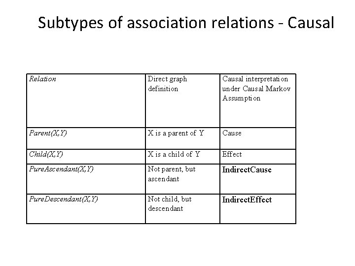
Subtypes of association relations - Causal Relation Direct graph definition Causal interpretation under Causal Markov Assumption Parent(X, Y) X is a parent of Y Cause Child(X, Y) X is a child of Y Effect Pure. Ascendant(X, Y) Not parent, but ascendant Indirect. Cause Pure. Descendant(X, Y) Not child, but descendant Indirect. Effect

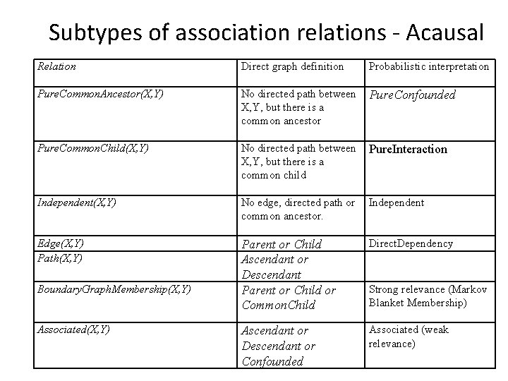
Subtypes of association relations - Acausal Relation Direct graph definition Probabilistic interpretation Pure. Common. Ancestor(X, Y) No directed path between X, Y, but there is a common ancestor Pure. Confounded Pure. Common. Child(X, Y) No directed path between X, Y, but there is a common child Pure. Interaction Independent(X, Y) No edge, directed path or common ancestor. Independent Edge(X, Y) Path(X, Y) Parent or Child Ascendant or Descendant Parent or Child or Common. Child Direct. Dependency Ascendant or Descendant or Confounded Associated (weak relevance) Boundary. Graph. Membership(X, Y) Associated(X, Y) Strong relevance (Markov Blanket Membership)

A more detailed language for associations: typed relevance

Aggregating to output • What can we do in case of multiple output? • E. g. Ig. E, Eosinophil, Rhinitis, Asthma. Status • Compute the posterior of „typed relevance” for – A given target, – Any of of the targets, – Excluding a given a target, – Being a multitarget. Note that typed relevance and typed output can be combined, though not arbitrarely.

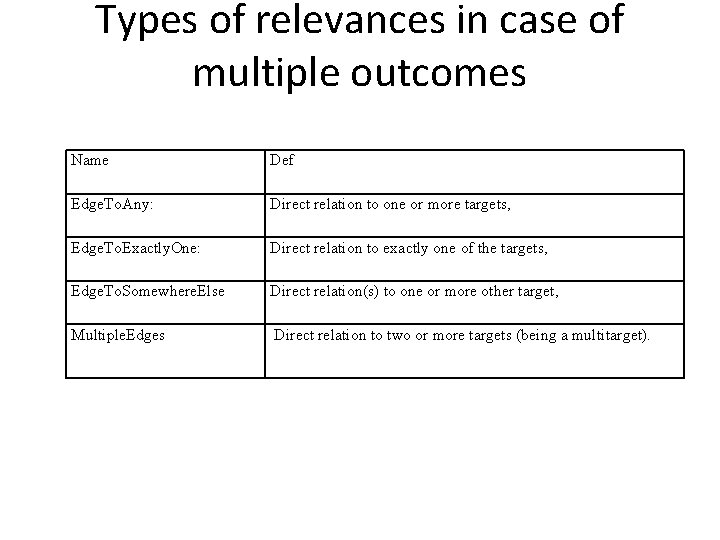
Types of relevances in case of multiple outcomes Name Def Edge. To. Any: Direct relation to one or more targets, Edge. To. Exactly. One: Direct relation to exactly one of the targets, Edge. To. Somewhere. Else Direct relation(s) to one or more other target, Multiple. Edges Direct relation to two or more targets (being a multitarget).

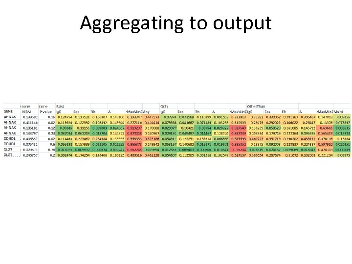
Aggregating to output

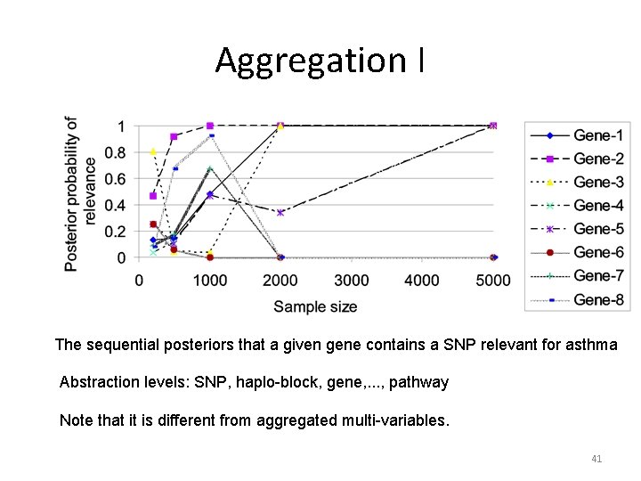
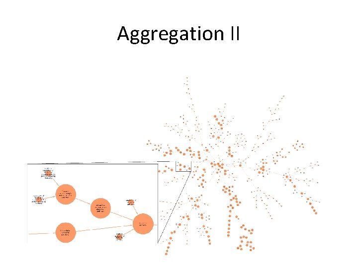
Aggregation I The sequential posteriors that a given gene contains a SNP relevant for asthma Abstraction levels: SNP, haplo-block, gene, . . . , pathway Note that it is different from aggregated multi-variables. 41

Aggregation II

Reporting • Optimal Bayesian decision about reporting – MBM – MBS • Decision theoretic approach

Summary • Challenges in biomarker discovery • Robustness (repeatability, transferability) • Causation • Multiple hypothesis testing • Interaction (multivariate approach) • Feature relevance • The feature subset selection problem • Identification of biomarkers • Methods – Challenges • Interpretation Bayesian networks • Causality Bayesian networks • Uncertainty Bayesian statistics • A Bayesian network based Bayesian approach to biomarker analysis