Intelligent Agents 1 dCNNs LSTMs ELMo Transformers BERT

Intelligent Agents 1 d-CNNs LSTMs ELMo Transformers BERT GPT Ralf Möller Universität zu Lübeck Institut für Informationssysteme

Acknowledgements • CS 546: Machine Learning in NLP (Spring 2020) – http: //courses. engr. illinois. edu/cs 546/ – Julia Hockenmaier http: //juliahmr. cs. illinois. edu – RNNs, LSTMs, ELMo, Transformers • Machine Learning (Spring 2020) – http: //speech. ee. ntu. edu. tw/~tlkagk/courses_ML 20. html – 李宏毅 (Hung-yi Lee ) http: //speech. ee. ntu. edu. tw/~tlkagk/ – ELMo, BERT: http: //speech. ee. ntu. edu. tw/~tlkagk/courses/ML_2019/Lecture/BERT%20(v 3). pdf 2

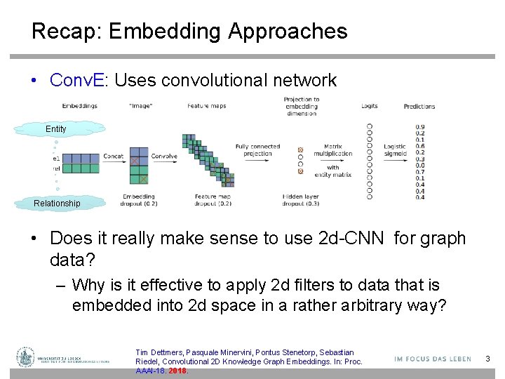
Recap: Embedding Approaches • Conv. E: Uses convolutional network Entity Relationship • Does it really make sense to use 2 d-CNN for graph data? – Why is it effective to apply 2 d filters to data that is embedded into 2 d space in a rather arbitrary way? Tim Dettmers, Pasquale Minervini, Pontus Stenetorp, Sebastian Riedel, Convolutional 2 D Knowledge Graph Embeddings. In: Proc. AAAI-18. 2018. 3

Recap: Convolution 4

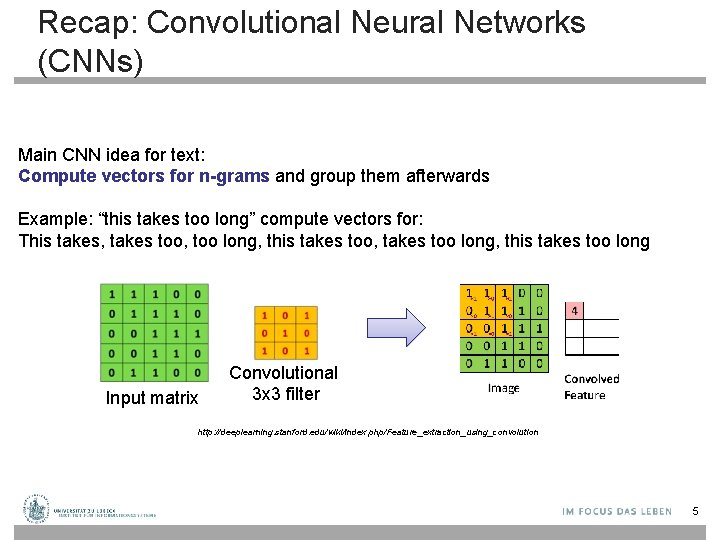
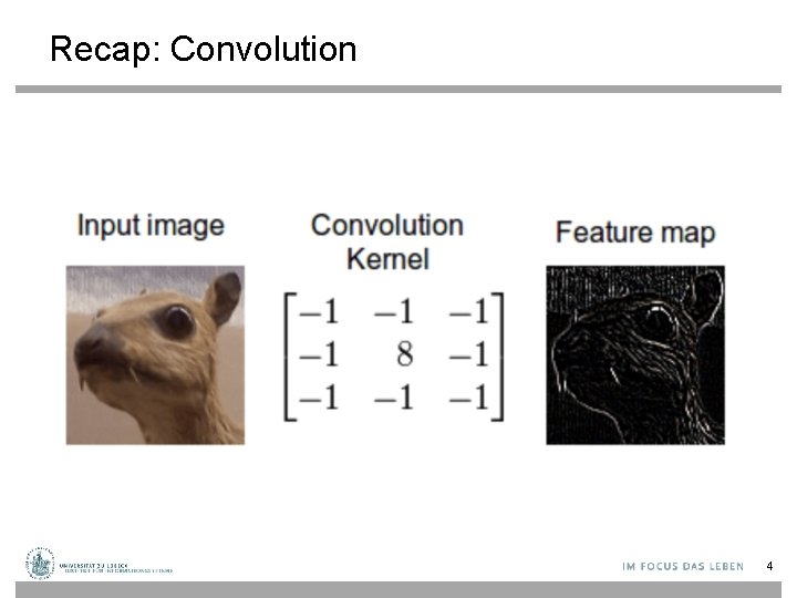
Recap: Convolutional Neural Networks (CNNs) Main CNN idea for text: Compute vectors for n-grams and group them afterwards Example: “this takes too long” compute vectors for: This takes, takes too, too long, this takes too, takes too long, this takes too long Input matrix Convolutional 3 x 3 filter http: //deeplearning. stanford. edu/wiki/index. php/Feature_extraction_using_convolution 5

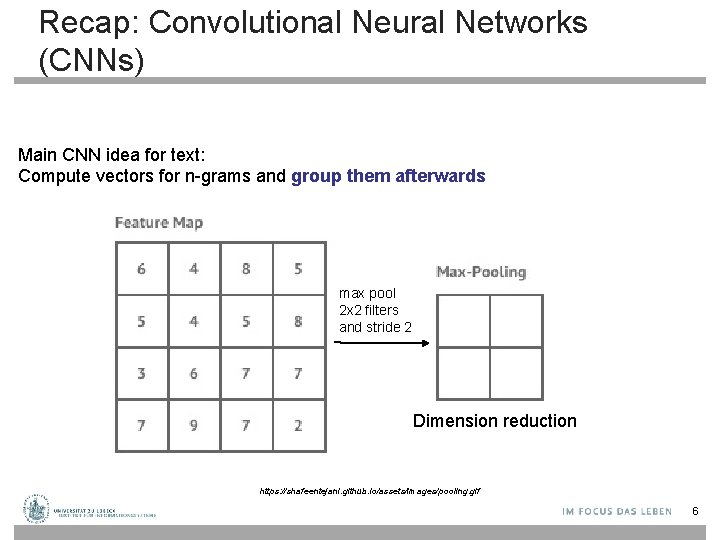
Recap: Convolutional Neural Networks (CNNs) Main CNN idea for text: Compute vectors for n-grams and group them afterwards max pool 2 x 2 filters and stride 2 Dimension reduction https: //shafeentejani. github. io/assets/images/pooling. gif 6

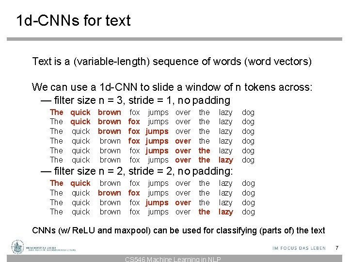
1 d-CNNs for text Text is a (variable-length) sequence of words (word vectors) We can use a 1 d-CNN to slide a window of n tokens across: — filter size n = 3, stride = 1, no padding The quick brown fox jumps over the The quick brown fox jumps over the lazy lazy dog dog dog — filter size n = 2, stride = 2, no padding: The quick brown fox jumps over the lazy dog dog CNNs (w/ Re. LU and maxpool) can be used for classifying (parts of) the text 7 CS 546 Machine Learning in NLP

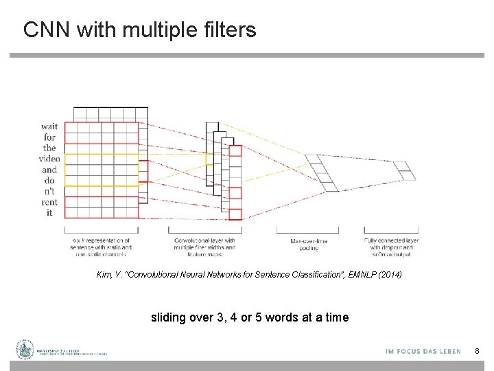
CNN with multiple filters Kim, Y. “Convolutional Neural Networks for Sentence Classification”, EMNLP (2014) sliding over 3, 4 or 5 words at a time 8

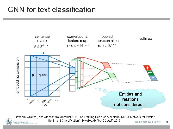
CNN for text classification Entities and relations not considered… Severyn, Aliaksei, and Alessandro Moschitti. "UNITN: Training Deep Convolutional Neural Network for Twitter Sentiment Classification. " Sem. Eval@ NAACL-HLT. 2015. 9

Fasttext (https: //fasttext. cc ) • Library for word embeddings and text classification o static word embeddings and ngram features o that get averaged together in one hidden layer o hierarchical softmax output over class labels • Enriching word vectors with subword information o Skipgram model where each word is a sum of character ngram embeddings and its own embedding o Each word is deterministically mapped to ngrams Piotr Bojanowski, Edouard Grave, Armand Joulin, Tomas Mikolov. Enriching Word Vectors with Subword Information. Transactions of the Association for Computational Linguistics, Volume 5. 135 -146. 2017. Armand Joulin, Edouard Grave, Piotr Bojanowski, Tomas Mikolov, Bag of Tricks for Efficient Text Classification. Proceedings of the 15 th Conference of the European Chapter of the Association for Computational Linguistics: Volume 2, Short Papers. 427 -431. 2017. Alon Jacovi, Oren Sar Shalom, Yoav Goldberg. Understanding Convolutional Neural Networks for Text Classification. In Proceedings of the 2018 EMNLP Workshop Blackbox. NLP: Analyzing and Interpreting Neural Networks for NLP. 2018. CS 546 Machine Learning in NLP 10

Multilingual Knowledge Graph Embeddings MTrans. E [Chen et al. 2017 a; 2017 b] ‐ Joint learning of structure encoders and an alignment model ‐ Alignment techniques: Linear transforms (best), vector translations, collocation (minimizing L 2 distance) JAPE [Sun et al. 2017] + Logistic‐based proximity normalizer for entity attributes ITrans. E [Zhu et al. 2017] ‐ self‐training + cross‐lingual collocation of entity embeddings KDCo. E [Chen et al. , 2018] leverages a weakly aligned multilingual KG for semi-supervised crosslingual learning using entity descriptions Boot. EA [Sun et al. , 2018] tries iteratively enlarge the labeled entity pairs based on the bootstrapping strategy 11

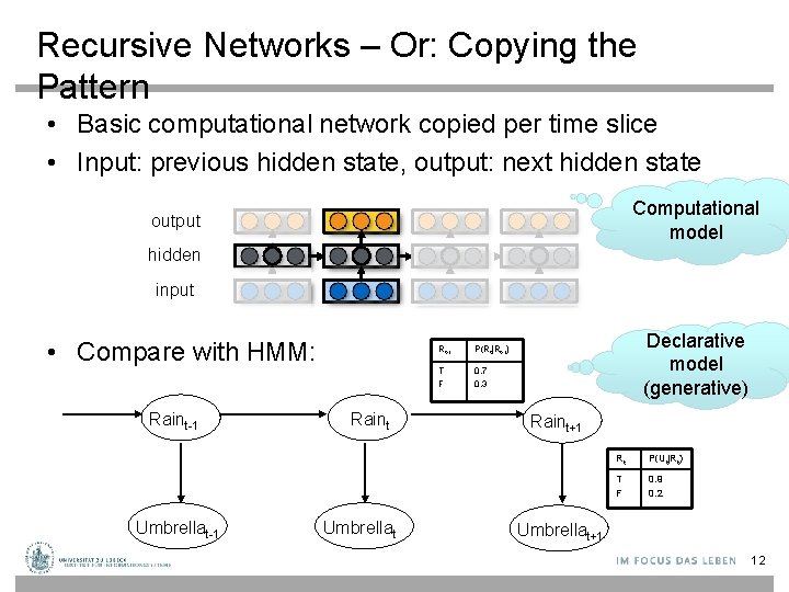
Recursive Networks – Or: Copying the Pattern • Basic computational network copied per time slice • Input: previous hidden state, output: next hidden state Computational model output hidden input • Compare with HMM: Raint-1 Umbrellat-1 Raint Umbrellat Rt-1 P(Rt|Rt-1) T F 0. 7 0. 3 Declarative model (generative) Raint+1 Rt P(Ut|Rt) T F 0. 9 0. 2 Umbrellat+1 12

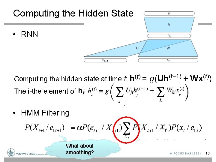
Computing the Hidden State • RNN Computing the hidden state at time t: h(t) = The i-the element of ht: hi(t) = g (∑ g(Uh(t− 1) + Wx(t)) Ujih (t− 1) + j j ) ∑ k Wki k ) x (t • HMM Filtering What about smoothing? 13

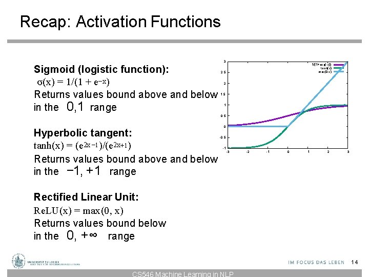
Recap: Activation Functions Sigmoid (logistic function): σ(x) = 1/(1 + e−x) Returns values bound above and below in the 0, 1 range 3 1/(1+exp(-x)) tanh(x) max(0, x) 2. 5 2 1. 5 1 0. 5 Hyperbolic tangent: tanh(x) = (e 2 x − 1)/(e 2 x+1) Returns values bound above and below in the − 1, +1 range 0 -0. 5 -1 -3 -2 -1 0 1 2 3 Rectified Linear Unit: Re. LU(x) = max(0, x) Returns values bound below in the 0, +∞ range 14 CS 546 Machine Learning in NLP

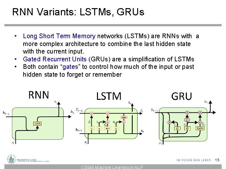
RNN Variants: LSTMs, GRUs • Long Short Term Memory networks (LSTMs) are RNNs with a more complex architecture to combine the last hidden state with the current input. • Gated Recurrent Units (GRUs) are a simplification of LSTMs • Both contain “gates” to control how much of the input or past hidden state to forget or remember 15 CS 546 Machine Learning in NLP

Gates • A gate performs element-wise multiplication of – the output of a d-dimensional sigmoid layer (all elements between 0 and 1), and – a d-dimensional input vector • Result: a d-dimensional output vector which is like the input, except some dimensions have been (partially) “forgotten” 16 CS 546 Machine Learning in NLP

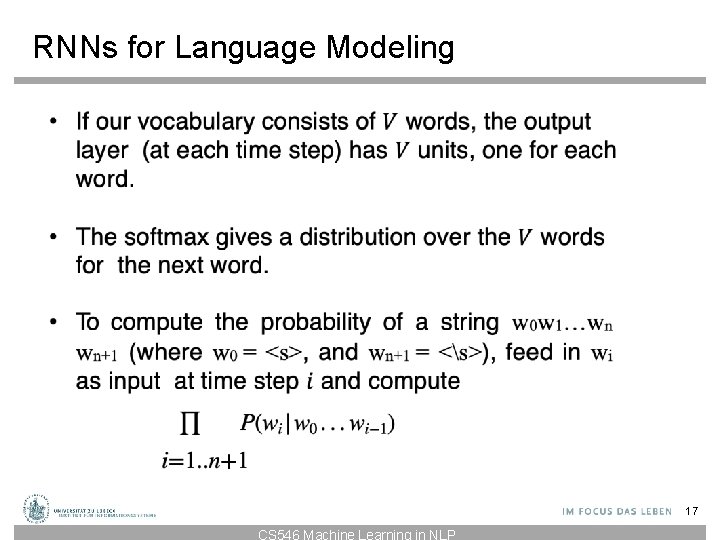
RNNs for Language Modeling 17 CS 546 Machine Learning in NLP

RNNs for Sequence Labeling • In sequence labeling, we want to assign a label or tag ti to each word wi • Now the output layer gives a distribution over the T possible tags. • The hidden layer contains information about the previous words and the previous tags. • To compute the probability of a tag sequence t 1…tn for a given string w 1…wn feed in wi (and possibly ti-1) as input at time step i and compute P(ti | w 1…wi-1, t 1…ti-1) 18 CS 546 Machine Learning in NLP

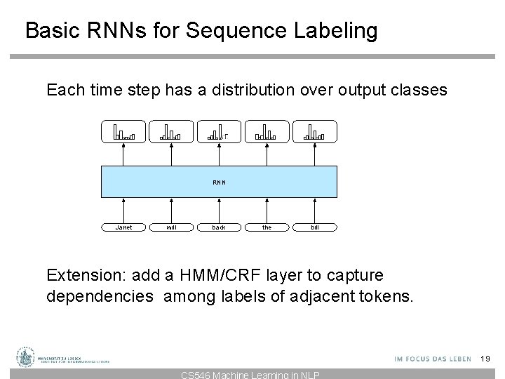
Basic RNNs for Sequence Labeling Each time step has a distribution over output classes RNN Janet will back the bill Extension: add a HMM/CRF layer to capture dependencies among labels of adjacent tokens. 19 CS 546 Machine Learning in NLP

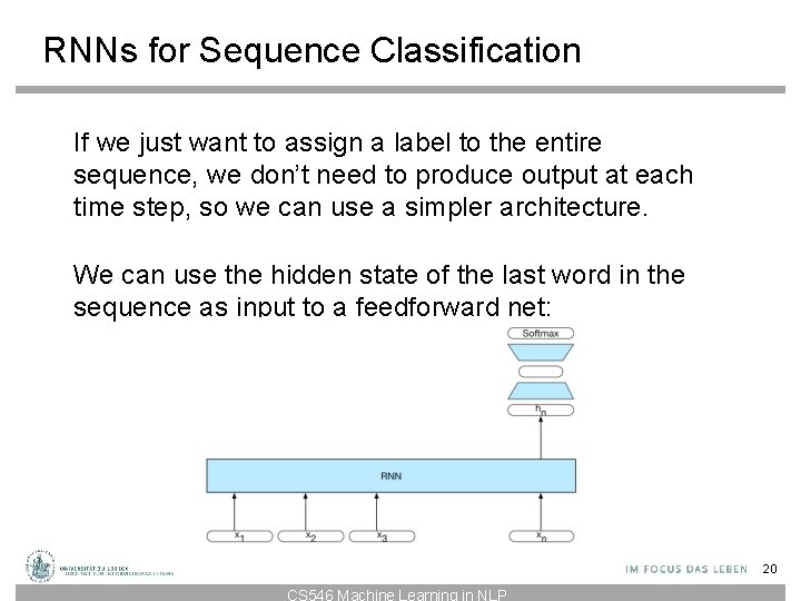
RNNs for Sequence Classification If we just want to assign a label to the entire sequence, we don’t need to produce output at each time step, so we can use a simpler architecture. We can use the hidden state of the last word in the sequence as input to a feedforward net: 20 CS 546 Machine Learning in NLP

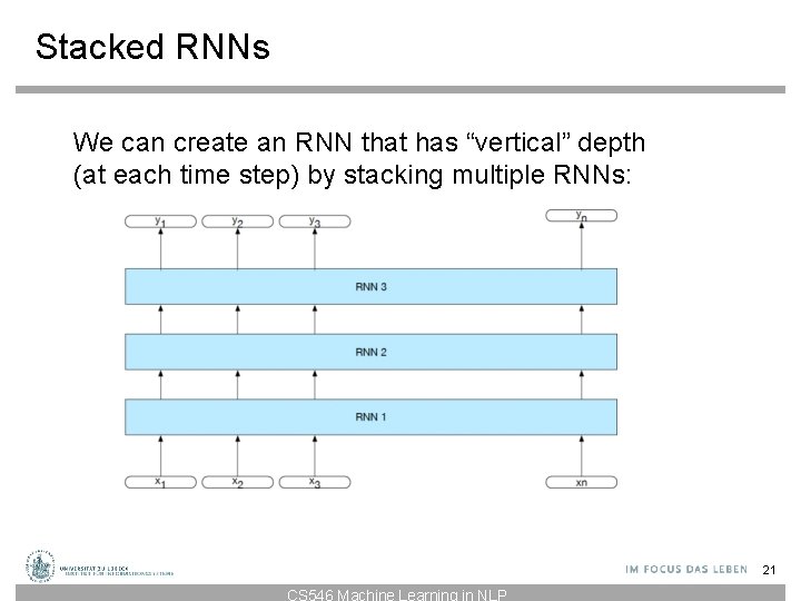
Stacked RNNs We can create an RNN that has “vertical” depth (at each time step) by stacking multiple RNNs: 21 CS 546 Machine Learning in NLP

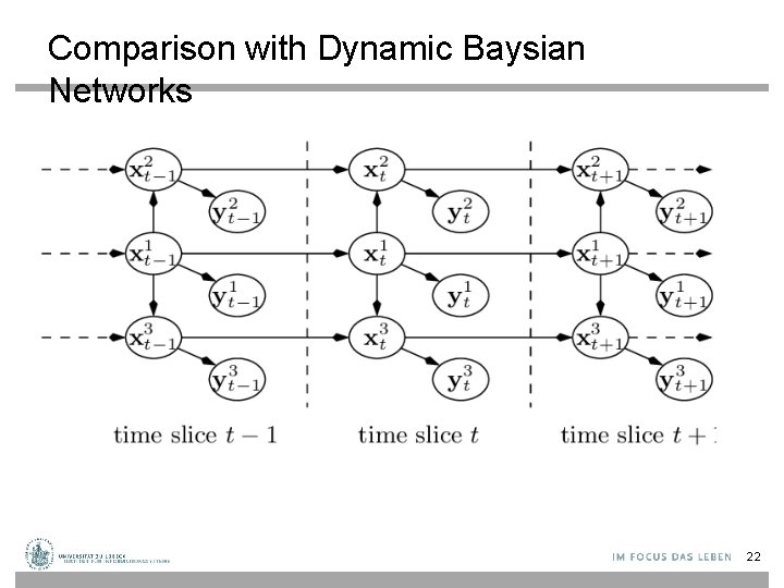
Comparison with Dynamic Baysian Networks 22

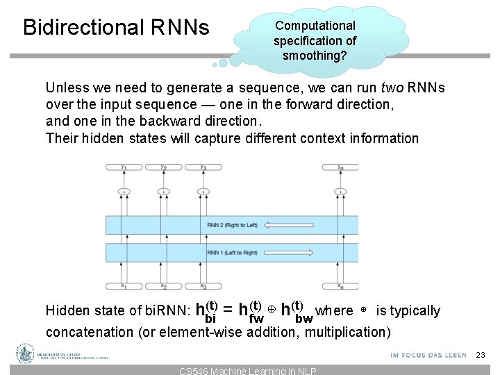
Bidirectional RNNs Computational specification of smoothing? Unless we need to generate a sequence, we can run two RNNs over the input sequence — one in the forward direction, and one in the backward direction. Their hidden states will capture different context information Hidden state of bi. RNN: h(t) bi (t) ⊕ h(t) where = hfw bw ⊕ is typically concatenation (or element-wise addition, multiplication) 23 CS 546 Machine Learning in NLP

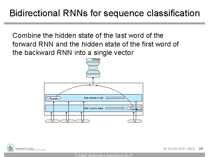
Bidirectional RNNs for sequence classification Combine the hidden state of the last word of the forward RNN and the hidden state of the first word of the backward RNN into a single vector Softmax + h 1_back RNN 2 (Right to Left) RNN 1 (Left to Right) x 1 x 2 hn_for w x 3 xn 24 CS 546 Machine Learning in NLP

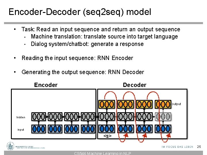
Encoder-Decoder (seq 2 seq) model • Task: Read an input sequence and return an output sequence • Machine translation: translate source into target language • Dialog system/chatbot: generate a response • Reading the input sequence: RNN Encoder • Generating the output sequence: RNN Decoder Encoder Decoder output hidden input <s> 25 CS 546 Machine Learning in NLP

Encoder-Decoder (seq 2 seq) Model Encoder RNN: reads in the input sequence passes its last hidden state to the initial hidden state of the decoder Decoder RNN: generates the output sequence typically uses different parameters from the encoder may also use different input embeddings 26 CS 546 Machine Learning in NLP

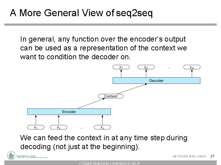
A More General View of seq 2 seq In general, any function over the encoder’s output can be used as a representation of the context we want to condition the decoder on. We can feed the context in at any time step during decoding (not just at the beginning). 27 CS 546 Machine Learning in NLP

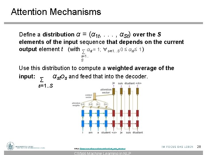
Attention Mechanisms Define a distribution α = (α 1 t, . . . , αSt) over the S elements of the input sequence that depends on the current output element t (with ∑ αst = 1; ∀s∈1. . . S 0 ≤ αst ≤ 1 ) s=1. . S Use this distribution to compute a weighted average of the input: ∑ αstos and feed that into the decoder. s=1. . S hhttps: //www. tensorflow. org/tutorials/text/nmt_with_attention CS 546 Machine Learning in NLP 28

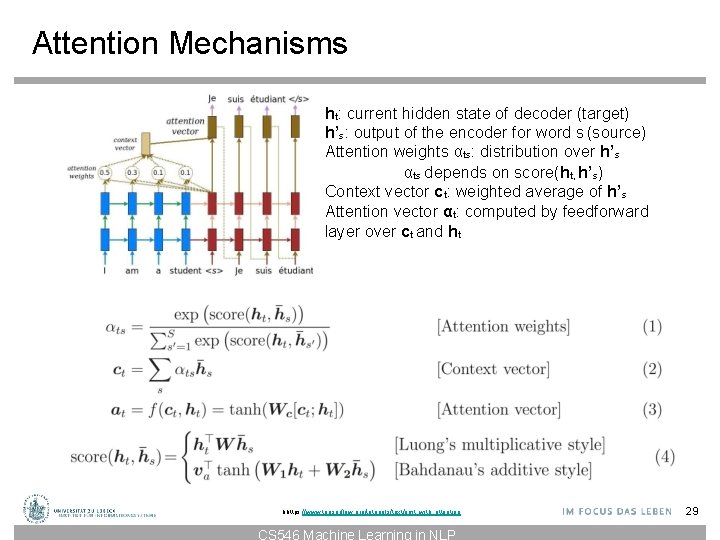
Attention Mechanisms ht: current hidden state of decoder (target) h’s: output of the encoder for word s (source) Attention weights αts: distribution over h’s αts depends on score(ht, h’s) Context vector ct: weighted average of h’s Attention vector αt: computed by feedforward layer over ct and ht hhttps: //www. tensorflow. org/tutorials/text/nmt_with_attention CS 546 Machine Learning in NLP 29

From RNNs to LSTMs • In simple RNNs, hidden state depends on previous hidden state and on the input: • ht = g(Wh[ht− 1, xt] + bh) with e. g. g=tanh • Vanishing gradient problem • RNNs can’t be trained effectively on long sequences • LSTMs (Long Short-Term Memory networks) to the rescue • Additional cell state passed through the network and updated at each time step • LSTMs define four different layers (gates) that read in the previous hidden state and current input. 30 CS 546 Machine Learning in NLP

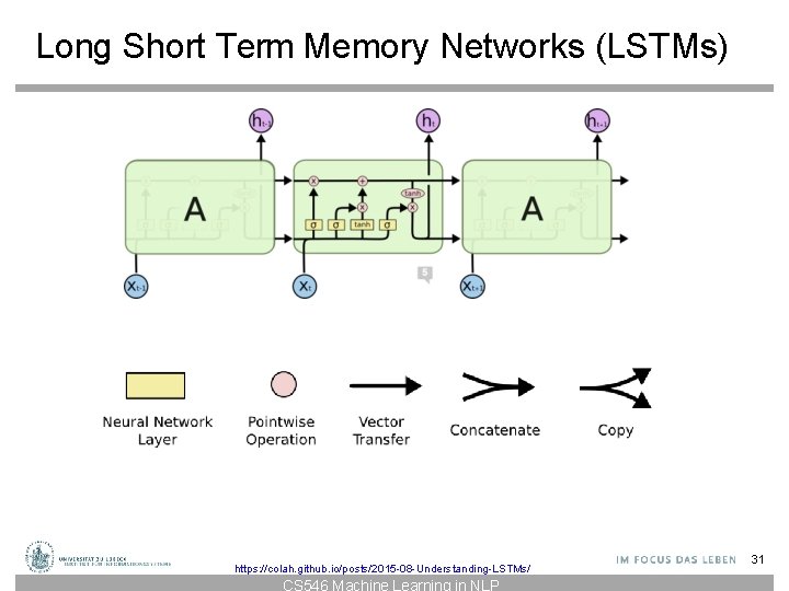
Long Short Term Memory Networks (LSTMs) https: //colah. github. io/posts/2015 -08 -Understanding-LSTMs/ CS 546 Machine Learning in NLP 31

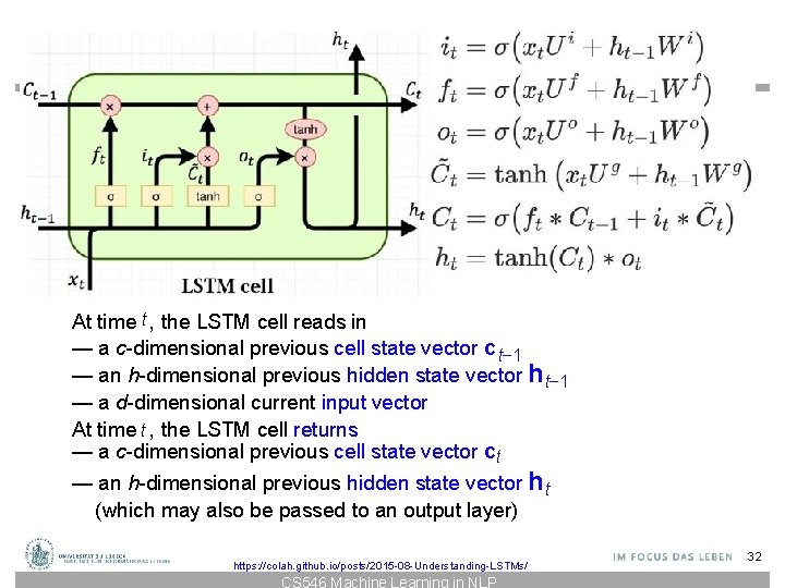
Long Short Term Memory Networks (LSTMs) At time t , the LSTM cell reads in — a c-dimensional previous cell state vector c t− 1 — an h-dimensional previous hidden state vector ht− 1 — a d-dimensional current input vector At time t , the LSTM cell returns — a c-dimensional previous cell state vector ct — an h-dimensional previous hidden state vector ht (which may also be passed to an output layer) https: //colah. github. io/posts/2015 -08 -Understanding-LSTMs/ CS 546 Machine Learning in NLP 32

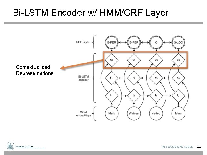
Bi-LSTM Encoder w/ HMM/CRF Layer Contextualized Representations 33

Embeddings from Language Models Replace static embeddings (lexicon lookup) with context-dependent embeddings (produced by a deep language model) => Each token’s representation is a function of the entire input sentence, computed by a deep (multi-layer) bidirectional language model => Return for each token a (task-dependent) linear combination of its representation across layers. => Different layers capture different information 34 CS 546 Machine Learning in NLP

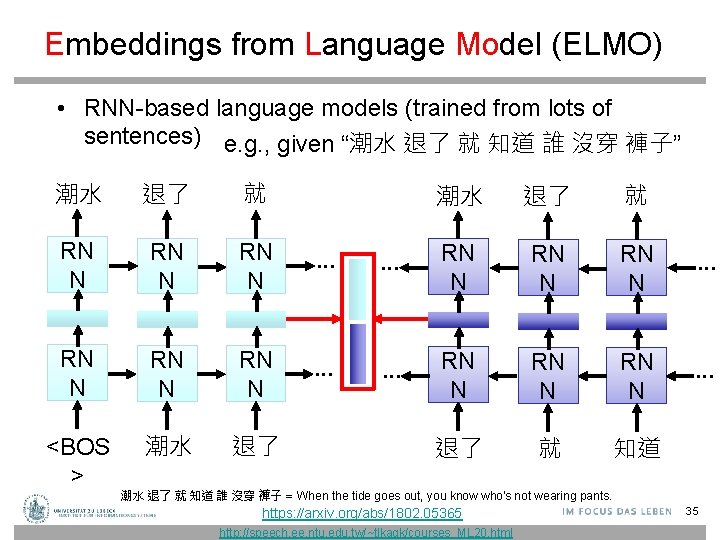
Embeddings from Language Model (ELMO) • RNN-based language models (trained from lots of sentences) e. g. , given “潮水 退了 就 知道 誰 沒穿 褲子” 潮水 退了 就 RN N RN N … <BOS > 潮水 退了 就 … RN N RN N … 退了 就 知道 潮水 退了 就 知道 誰 沒穿 褲子 = When the tide goes out, you know who's not wearing pants. https: //arxiv. org/abs/1802. 05365 http: //speech. ee. ntu. edu. tw/~tlkagk/courses_ML 20. html 35

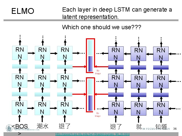
Each layer in deep LSTM can generate a latent representation. ELMO Which one should we use? ? ? … … … RN N RN N RN N … RN N RN N … <BOS > 潮水 退了 退了 就 知道 http: //speech. ee. ntu. edu. tw/~tlkagk/courses_ML 20. html 36

ELMo architecture • Train a multi-layer bidirectional language model with character convolutions on raw text • Each layer of this language model network computes a vector representation for each token. • Freeze the parameters of the language model. • For each task: train task-dependent softmax weights to combine the layer-wise representations into a single vector for each token jointly with a task-specific model that uses those vectors 37 CS 546 Machine Learning in NLP

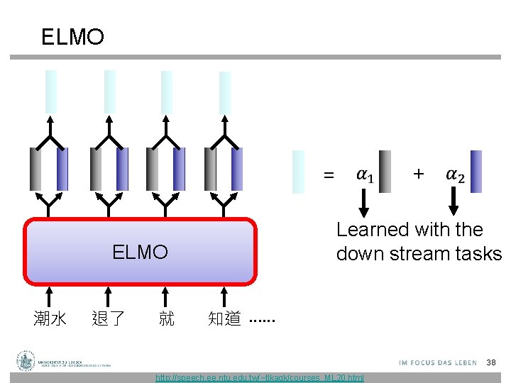
ELMO + = Learned with the down stream tasks ELMO 潮水 退了 就 知道 …… 38 http: //speech. ee. ntu. edu. tw/~tlkagk/courses_ML 20. html

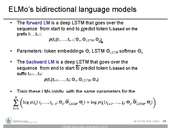
ELMo’s bidirectional language models • The forward LM is a deep LSTM that goes over the sequence from start to end to predict token tk based on the prefix t 1…tk-1: p(tk | t 1, …, tk− 1; Θx, ΘLSTM, Θs) • Parameters: token embeddings Θx LSTM ΘLSTM softmax Θs • The backward LM is a deep LSTM that goes over the sequence from end to start to predict token tk based on the suffix tk+1…t. N: p(tk | tk+1, …, t. N; Θx, ΘLSTM, Θs) • Train these LMs jointly, with the same parameters for the Ntoken representations and the softmax layer (but not for the log p(t | t , …, k− 1 t ; Θx , ΘLSTM, Θs ) + log p(tk | tk+1, …, Nt ; Θx , ΘLSTM, Θ ) ∑ LSTMs) k 1 k=1 ( ) s 39 CS 546 Machine Learning in NLP

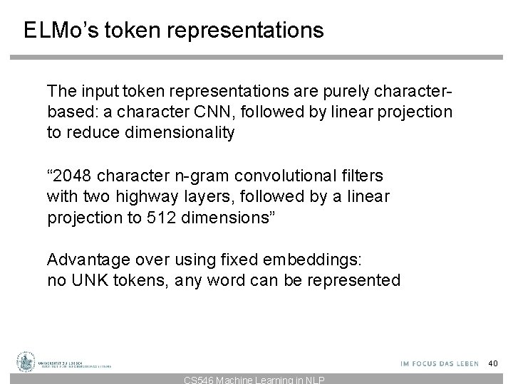
ELMo’s token representations The input token representations are purely characterbased: a character CNN, followed by linear projection to reduce dimensionality “ 2048 character n-gram convolutional filters with two highway layers, followed by a linear projection to 512 dimensions” Advantage over using fixed embeddings: no UNK tokens, any word can be represented 40 CS 546 Machine Learning in NLP

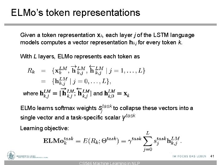
ELMo’s token representations Given a token representation xk, each layer j of the LSTM language models computes a vector representation hk, j for every token k. With L layers, ELMo represents each token as ELMo learns softmax weights sjtask to collapse these vectors into a single vector and a task-specific scalar γtask Learning objective: 41 CS 546 Machine Learning in NLP

Weighted Softmax [Wikipedia] 42

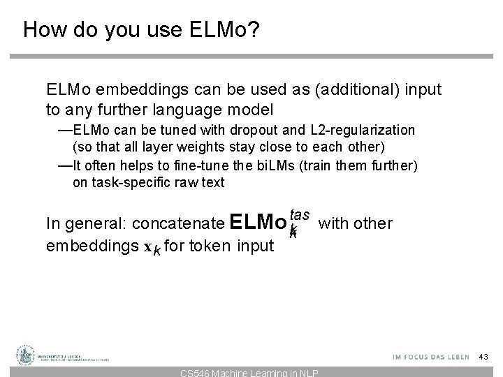
How do you use ELMo? ELMo embeddings can be used as (additional) input to any further language model —ELMo can be tuned with dropout and L 2 -regularization (so that all layer weights stay close to each other) —It often helps to fine-tune the bi. LMs (train them further) on task-specific raw text tas In general: concatenate ELMo k k embeddings xk for token input with other 43 CS 546 Machine Learning in NLP

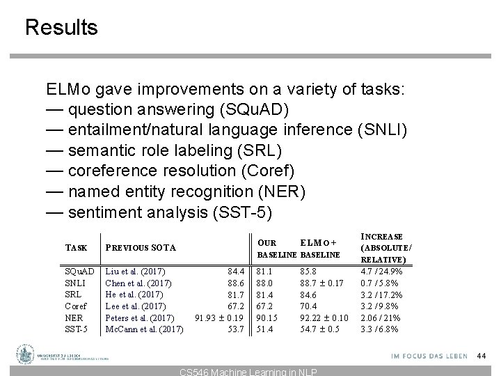
Results ELMo gave improvements on a variety of tasks: — question answering (SQu. AD) — entailment/natural language inference (SNLI) — semantic role labeling (SRL) — coreference resolution (Coref) — named entity recognition (NER) — sentiment analysis (SST-5) O UR TASK P REVIOUS SOTA SQu. AD SNLI SRL Coref NER SST-5 Liu et al. (2017) Chen et al. (2017) He et al. (2017) Lee et al. (2017) Peters et al. (2017) Mc. Cann et al. (2017) ELM O + BASELINE 84. 4 88. 6 81. 7 67. 2 91. 93 ± 0. 19 53. 7 81. 1 88. 0 81. 4 67. 2 90. 15 51. 4 85. 8 88. 7 ± 0. 17 84. 6 70. 4 92. 22 ± 0. 10 54. 7 ± 0. 5 I NCREASE ( ABSOLUTE / RELATIVE ) 4. 7 / 24. 9% 0. 7 / 5. 8% 3. 2 / 17. 2% 3. 2 / 9. 8% 2. 06 / 21% 3. 3 / 6. 8% 44 CS 546 Machine Learning in NLP

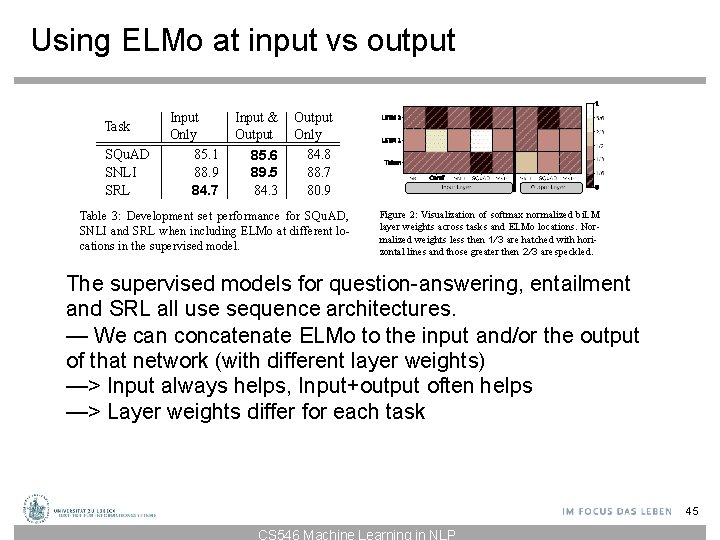
Using ELMo at input vs output Task SQu. AD SNLI SRL Input Only 85. 1 88. 9 84. 7 Input & Output Only 85. 6 89. 5 84. 3 84. 8 88. 7 80. 9 Table 3: Development set performance for SQu. AD, SNLI and SRL when including ELMo at different locations in the supervised model. Figure 2: Visualization of softmax normalized bi. LM layer weights across tasks and ELMo locations. Normalized weights less then 1/3 are hatched with horizontal lines and those greater then 2/3 are speckled. The supervised models for question-answering, entailment and SRL all use sequence architectures. — We can concatenate ELMo to the input and/or the output of that network (with different layer weights) —> Input always helps, Input+output often helps —> Layer weights differ for each task 45 CS 546 Machine Learning in NLP

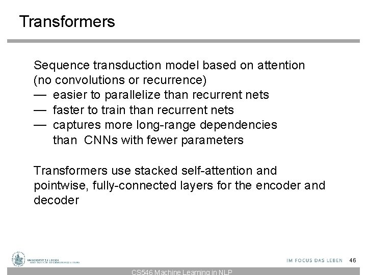
Transformers Sequence transduction model based on attention (no convolutions or recurrence) — easier to parallelize than recurrent nets — faster to train than recurrent nets — captures more long-range dependencies than CNNs with fewer parameters Transformers use stacked self-attention and pointwise, fully-connected layers for the encoder and decoder 46 CS 546 Machine Learning in NLP

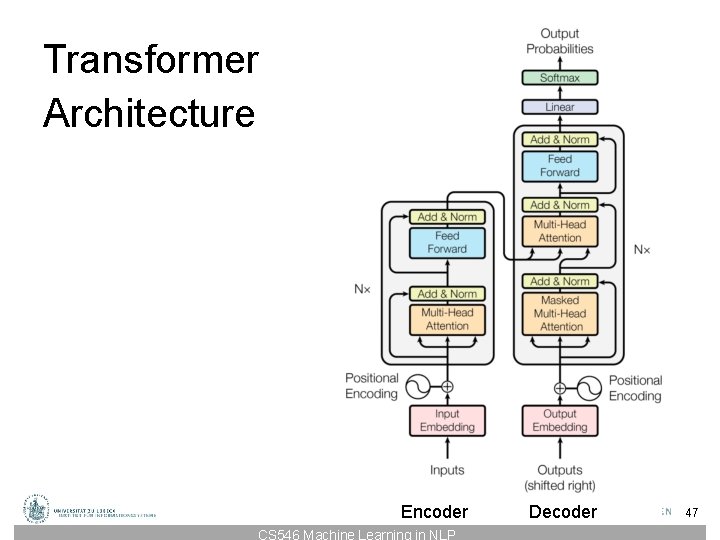
Transformer Architecture Encoder CS 546 Machine Learning in NLP Decoder 47

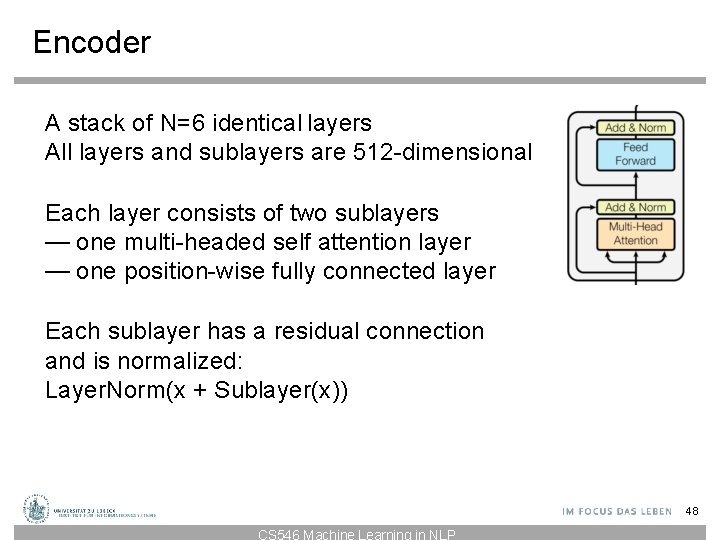
Encoder A stack of N=6 identical layers All layers and sublayers are 512 -dimensional Each layer consists of two sublayers — one multi-headed self attention layer — one position-wise fully connected layer Each sublayer has a residual connection and is normalized: Layer. Norm(x + Sublayer(x)) 48 CS 546 Machine Learning in NLP

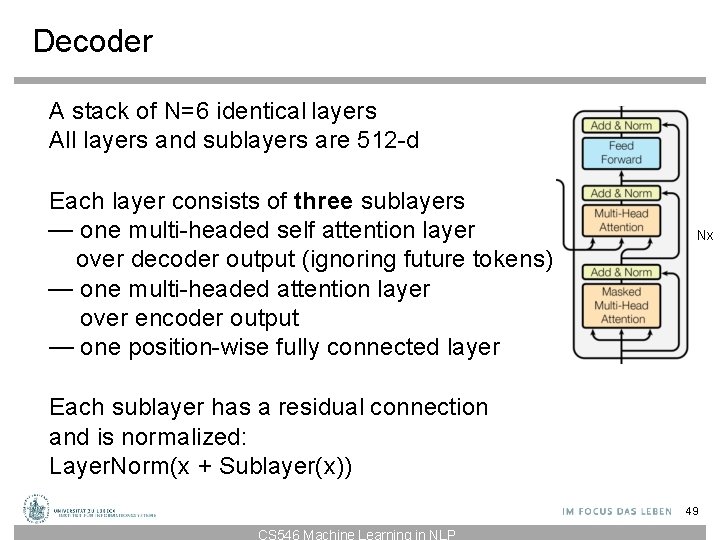
Decoder A stack of N=6 identical layers All layers and sublayers are 512 -d Each layer consists of three sublayers — one multi-headed self attention layer over decoder output (ignoring future tokens) — one multi-headed attention layer over encoder output — one position-wise fully connected layer Nx Each sublayer has a residual connection and is normalized: Layer. Norm(x + Sublayer(x)) 49 CS 546 Machine Learning in NLP

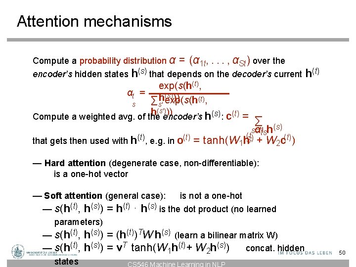
Attention mechanisms Compute a probability distribution α = (α 1 t, . . . , αSt) over the encoder’s hidden states h(s) that depends on the decoder’s current h(t) exp(s(h(t), αt = h(s))) ∑s′ exp(s(h(t), s h(s′)encoder’s )) Compute a weighted avg. of the h(s): c(t) = ∑ that gets then used with h(t), e. g. in o(t) = αtsh(s) s=1. . tanh(W 1 h(t. S) + W 2 c(t)) — Hard attention (degenerate case, non-differentiable): is a one-hot vector — Soft attention (general case): is not a one-hot — s(h(t), h(s)) = h(t) ⋅ h(s) is the dot product (no learned parameters) — s(h(t), h(s)) = (h(t))TW h(s) (learn a bilinear matrix W) — s(h(t), h(s)) = v. T tanh(W 1 h(t) + W 2 h(s)) concat. hidden states CS 546 Machine Learning in NLP 50

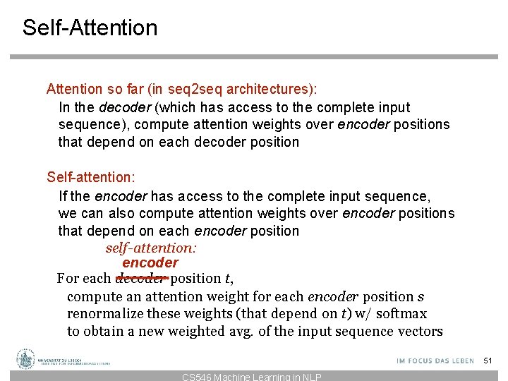
Self-Attention so far (in seq 2 seq architectures): In the decoder (which has access to the complete input sequence), compute attention weights over encoder positions that depend on each decoder position Self-attention: If the encoder has access to the complete input sequence, we can also compute attention weights over encoder positions that depend on each encoder position self-attention: encoder For each decoder position t, compute an attention weight for each encoder position s renormalize these weights (that depend on t) w/ softmax to obtain a new weighted avg. of the input sequence vectors 51 CS 546 Machine Learning in NLP

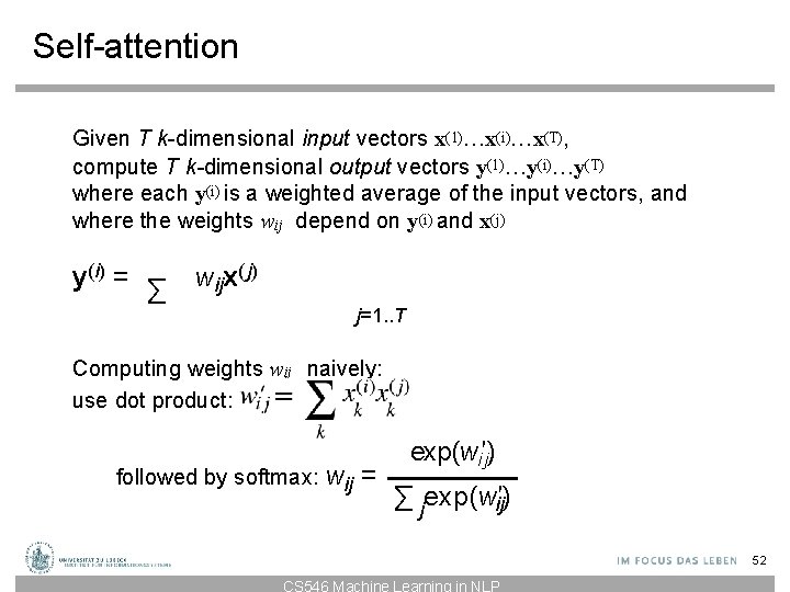
Self-attention Given T k-dimensional input vectors x(1)…x(i)…x(T), compute T k-dimensional output vectors y(1)…y(i)…y(T) where each y(i) is a weighted average of the input vectors, and where the weights wij depend on y(i) and x(j) y (i ) = ∑ wijx( j) j=1. . T Computing weights wij naively: x (i)x ( j) use dot product: wi′j = ∑ k k followed by softmax: wij = k exp(wi′j) ∑ jexp(w′) ij 52 CS 546 Machine Learning in NLP

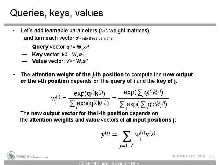
Queries, keys, values • Let’s add learnable parameters (kxk weight matrices), and turn each vector x(i) into three versions: — Query vector q(i) = Wqx(i) — Key vector: k(i) = Wkx(i) — Value vector: v(i) = Wvx(i) • The attention weight of the j-th position to compute the new output or the i-th position depends on the query of i and the key of j: (i)k( j)) exp( ∑l ql(i)kl( j)) exp(q wj(i) = = (i) ( j) ∑ jexp(q k ) ∑ jexp( ∑ lq(i) l kl ) The new output vector for the i-th position depends on the attention weights and value vectors of all input positions j: y(i) = ∑ wj(i)v( j) j=1. . T 53 CS 546 Machine Learning in NLP

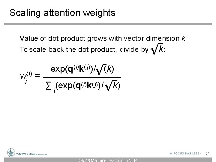
Scaling attention weights Value of dot product grows with vector dimension k To scale back the dot product, divide by wj(i) = k: exp(q(i)k( j))/ (k) ∑ j (exp(q(i)k( j))/ k) 54 CS 546 Machine Learning in NLP

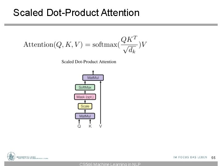
Scaled Dot-Product Attention 55 CS 546 Machine Learning in NLP

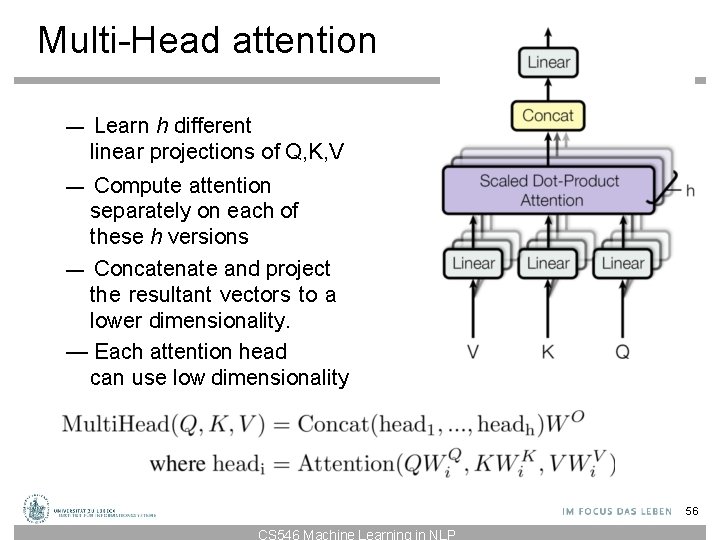
Multi-Head attention — Learn h different linear projections of Q, K, V — Compute attention separately on each of these h versions — Concatenate and project the resultant vectors to a lower dimensionality. — Each attention head can use low dimensionality 56 CS 546 Machine Learning in NLP

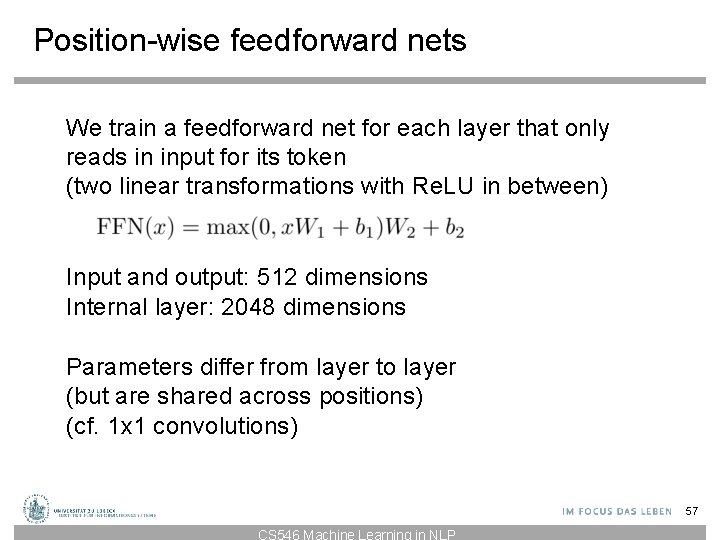
Position-wise feedforward nets We train a feedforward net for each layer that only reads in input for its token (two linear transformations with Re. LU in between) Input and output: 512 dimensions Internal layer: 2048 dimensions Parameters differ from layer to layer (but are shared across positions) (cf. 1 x 1 convolutions) 57 CS 546 Machine Learning in NLP

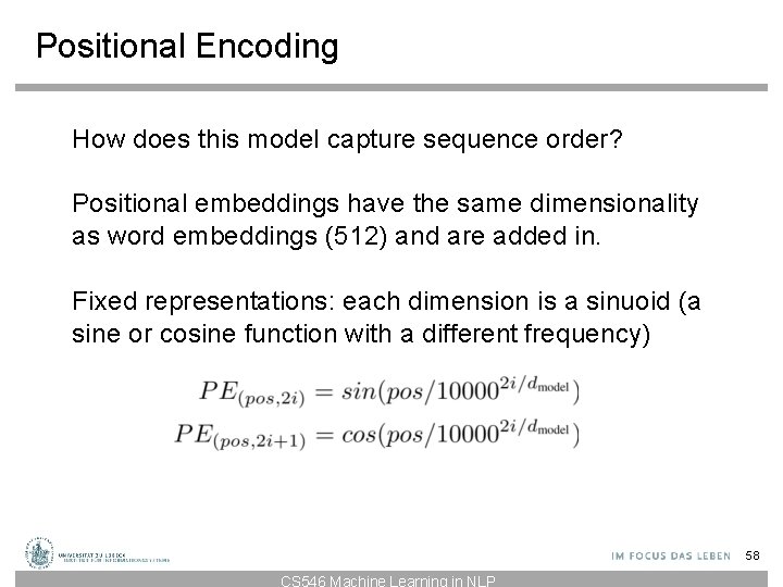
Positional Encoding How does this model capture sequence order? Positional embeddings have the same dimensionality as word embeddings (512) and are added in. Fixed representations: each dimension is a sinuoid (a sine or cosine function with a different frequency) 58 CS 546 Machine Learning in NLP

A word can have multiple senses. Have you paid that money to the bank yet ? It is safest to deposit your money in the bank. The victim was found lying dead on the river bank. They stood on the river bank to fish. The hospital has its own blood bank. The third sense or not? https: //arxiv. org/abs/1902. 06006 http: //speech. ee. ntu. edu. tw/~tlkagk/courses_ML 20. html 59

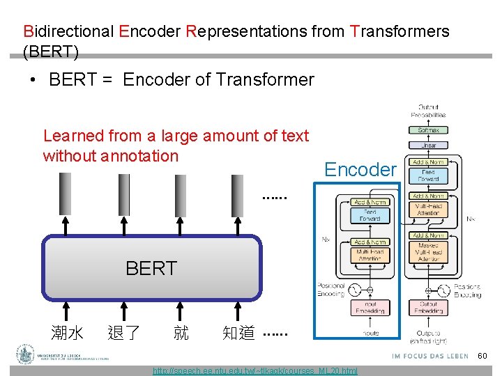
Bidirectional Encoder Representations from Transformers (BERT) • BERT = Encoder of Transformer Learned from a large amount of text without annotation Encoder …… BERT 潮水 退了 就 知道 …… 60 http: //speech. ee. ntu. edu. tw/~tlkagk/courses_ML 20. html

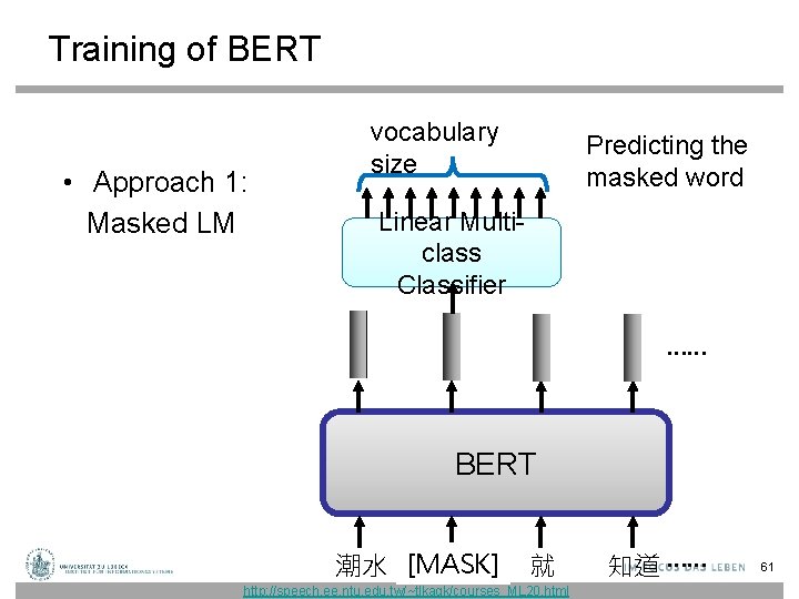
Training of BERT • Approach 1: Masked LM vocabulary size Predicting the masked word Linear Multiclass Classifier …… BERT 潮水 [MASK] 退了 就 http: //speech. ee. ntu. edu. tw/~tlkagk/courses_ML 20. html 知道 …… 61

Training of BERT Approach 2: Next Sentence Prediction [CLS]: the position that outputs classification results [SEP]: the boundary of two sentences Approaches 1 and 2 are used at the same time. yes Linear Binary Classifier BERT [CLS] 醒醒 吧 [SEP] 你 沒有 妹妹 62 http: //speech. ee. ntu. edu. tw/~tlkagk/courses_ML 20. html

Training of BERT Approach 2: Next Sentence Prediction [CLS]: the position that outputs classification results [SEP]: the boundary of two sentences Approaches 1 and 2 are used at the same time. No Linear Binary Classifier BERT [CLS] 醒醒 吧 [SEP] 眼睛 業障 重 63 http: //speech. ee. ntu. edu. tw/~tlkagk/courses_ML 20. html

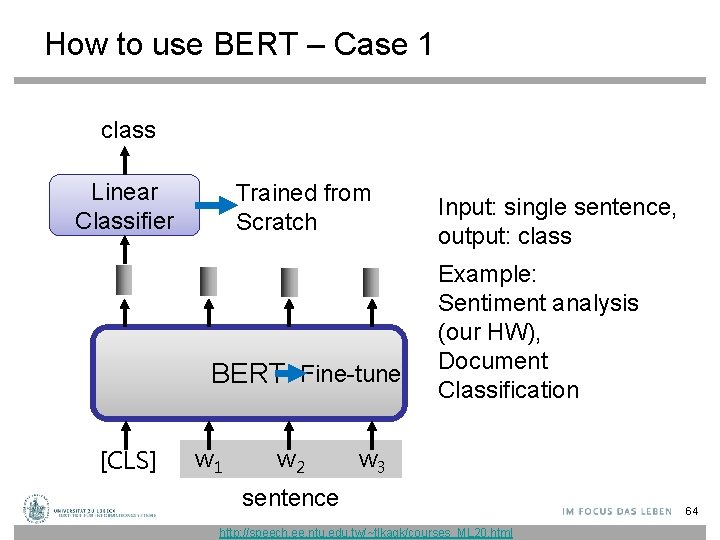
How to use BERT – Case 1 class Linear Classifier Trained from Scratch BERT Fine-tune [CLS] w 1 w 2 Input: single sentence, output: class Example: Sentiment analysis (our HW), Document Classification w 3 sentence http: //speech. ee. ntu. edu. tw/~tlkagk/courses_ML 20. html 64

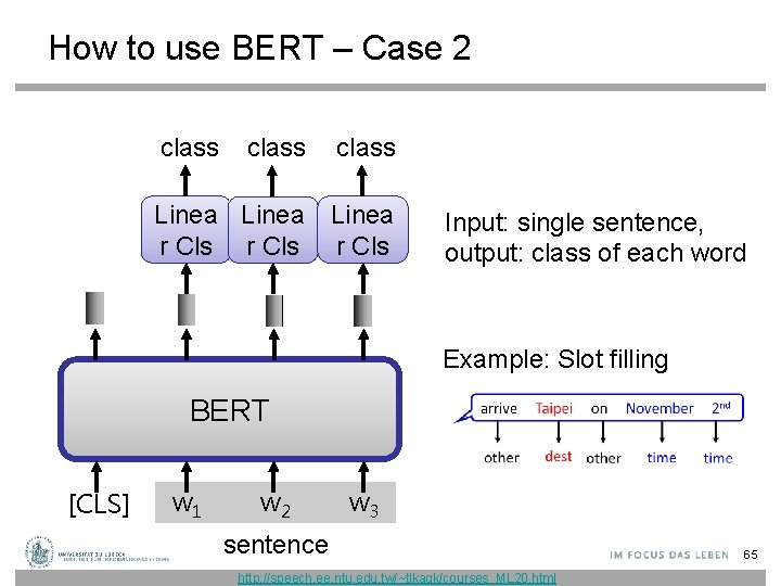
How to use BERT – Case 2 class Linea r Cls Input: single sentence, output: class of each word Example: Slot filling BERT [CLS] w 1 w 2 w 3 sentence http: //speech. ee. ntu. edu. tw/~tlkagk/courses_ML 20. html 65

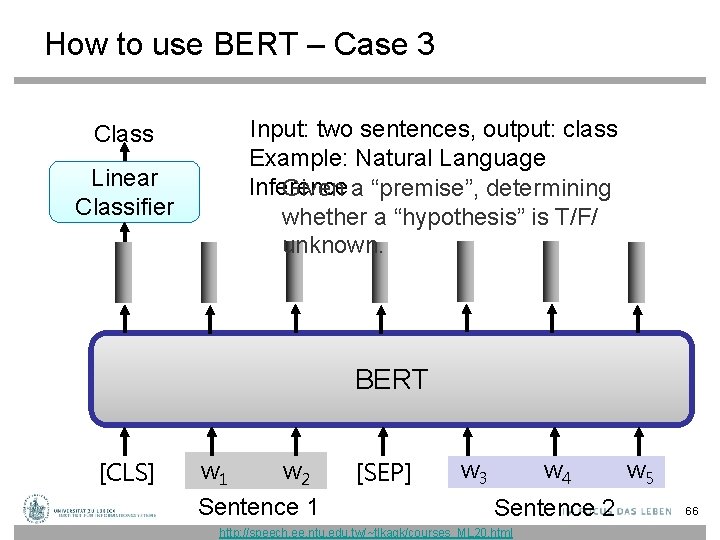
How to use BERT – Case 3 Input: two sentences, output: class Example: Natural Language Inference Given a “premise”, determining whether a “hypothesis” is T/F/ unknown. Class Linear Classifier BERT [CLS] w 1 w 2 Sentence 1 [SEP] w 3 w 4 Sentence 2 http: //speech. ee. ntu. edu. tw/~tlkagk/courses_ML 20. html w 5 66

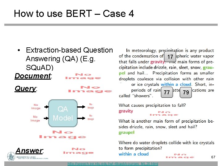
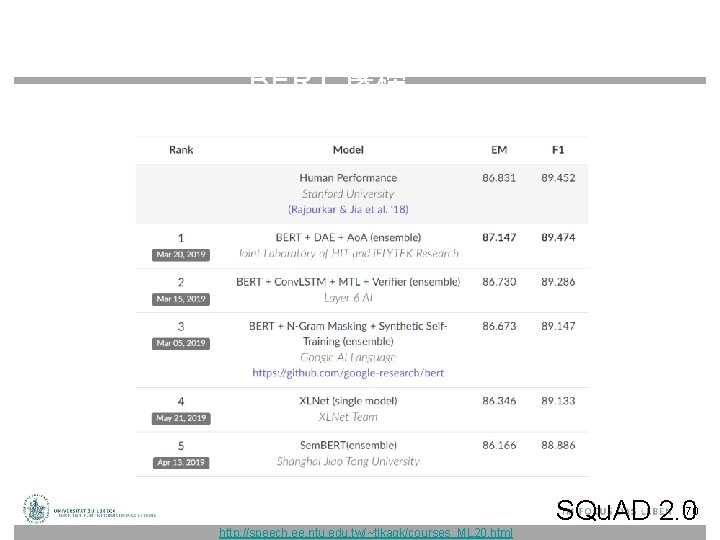
How to use BERT – Case 4 • Extraction-based Question Answering (QA) (E. g. SQu. AD) Document: Query: 17 77 79 QA Model Answer: 67 http: //speech. ee. ntu. edu. tw/~tlkagk/courses_ML 20. html

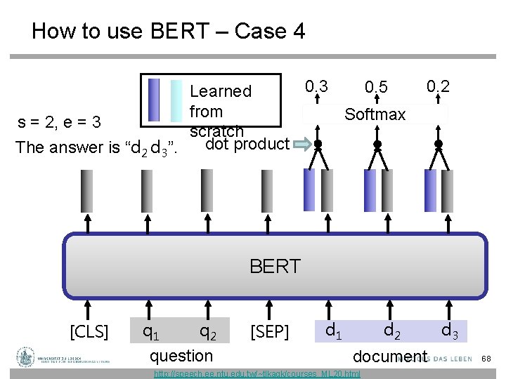
How to use BERT – Case 4 0. 3 0. 5 Learned from Softmax s = 2, e = 3 scratch dot product The answer is “d 2 d 3”. 0. 2 BERT [CLS] q 1 q 2 question [SEP] d 1 d 2 document http: //speech. ee. ntu. edu. tw/~tlkagk/courses_ML 20. html d 3 68

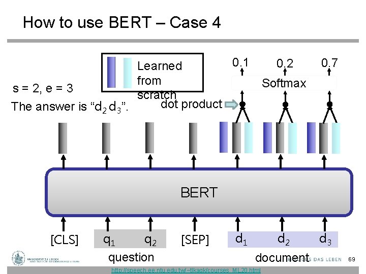
How to use BERT – Case 4 0. 1 0. 2 Learned from Softmax s = 2, e = 3 scratch dot product The answer is “d 2 d 3”. 0. 7 BERT [CLS] q 1 q 2 question [SEP] d 1 d 2 document http: //speech. ee. ntu. edu. tw/~tlkagk/courses_ML 20. html d 3 69

BERT 屠榜 …… SQu. AD 2. 0 70 http: //speech. ee. ntu. edu. tw/~tlkagk/courses_ML 20. html

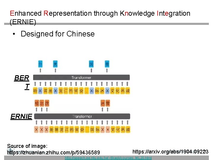
Enhanced Representation through Knowledge Integration (ERNIE) • Designed for Chinese BER T ERNIE Source of image: https: //zhuanlan. zhihu. com/p/59436589 71 https: //arxiv. org/abs/1904. 09223 http: //speech. ee. ntu. edu. tw/~tlkagk/courses_ML 20. html

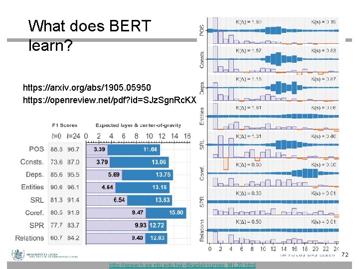
What does BERT learn? https: //arxiv. org/abs/1905. 05950 https: //openreview. net/pdf? id=SJz. Sgn. Rc. KX 72 http: //speech. ee. ntu. edu. tw/~tlkagk/courses_ML 20. html

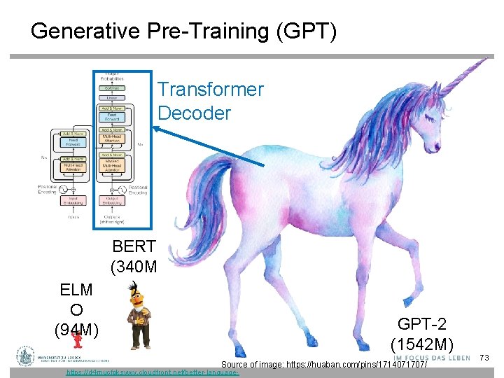
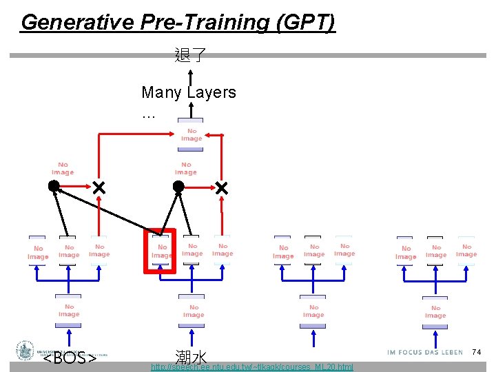
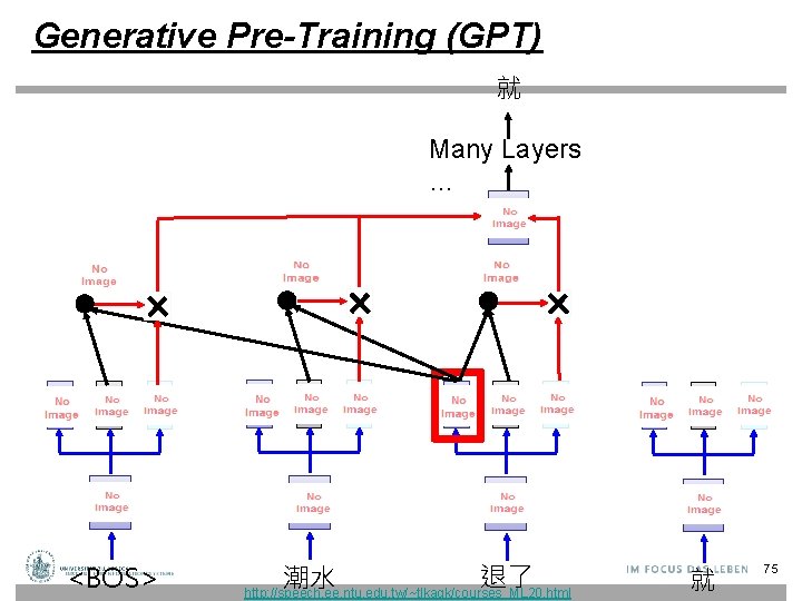
Generative Pre-Training (GPT) Transformer Decoder BERT (340 M ) ELM O (94 M) GPT-2 (1542 M) Source of image: https: //huaban. com/pins/1714071707/ https: //d 4 mucfpksywv. cloudfront. net/better-language- 73

Generative Pre-Training (GPT) 退了 Many Layers … <BOS> 潮水 http: //speech. ee. ntu. edu. tw/~tlkagk/courses_ML 20. html 74

Generative Pre-Training (GPT) 就 Many Layers … <BOS> 退了 潮水 http: //speech. ee. ntu. edu. tw/~tlkagk/courses_ML 20. html 就 75

Zero-shot Learning? • Reading Comprehension Co. QA • Summarization • Translation English sentence = French sentence 1 1 English sentence = French sentence 2 2 English sentence = 76 http: //speech. ee. ntu. edu. tw/~tlkagk/courses_ML 20. html

Visualization https: //arxiv. org/abs/1904. 02679 (The results below are from GPT-2) 77 http: //speech. ee. ntu. edu. tw/~tlkagk/courses_ML 20. html

BERT as a Markov Random Field Language Model • Show that BERT (Devlin et al. , 2018) is a Markov random field language model • Gives way to a natural procedure to sample sentences from BERT – Can produce high quality, fluent generations – Generates sentences that are more diverse but of slightly worse quality Alex Wang, Kyunghyun Cho. BERT has a Mouth, and It Must Speak: BERT as a Markov Random Field Language Model. Volume: In Proc. of the Workshop on Methods for Optimizing and Evaluating Neural Language Generation, June 2019. https: //arxiv. org/abs/1902. 04094 http: //speech. ee. ntu. edu. tw/~tlkagk/courses_ML 20. html 78