Intel OPEN SOURCE COMPUTER VISION LIBRARY Goals n

Intel® OPEN SOURCE COMPUTER VISION LIBRARY

Goals n Develop a universal toolbox for research and development in the field of Computer Vision

We will talk about: n Algorithmic content n Technical content n Examples of usage n Trainings

Open. CV algorithms

Open. CV Functionality (more than 350 algorithms) n n n Basic structures and operations Image Analysis Structural Analysis Object Recognition Motion Analysis and Object Tracking 3 D Reconstruction

Basic Structures and Operations n n Multidimensional array operations Dynamic structures operations Drawing primitives Utility functions Victor Eruhimov: Multidimensional array operations include operations on images, matrices and histograms. In the future, when I talk about image operations, keep in mind that all operations are applicable to matrices and histograms as well. Dynamic structures operations concern all vector data storages. They will be discussed in detail in the Technical Section. Drawing primitives allows not only to draw primitives but to use the algorithms for pixel access. Utility functions, in particular, contain fast implementations of useful math functions.

Image Analysis n n n n Thresholds Statistics Pyramids Morphology Distance transform Flood fill Feature detection Contours retrieving

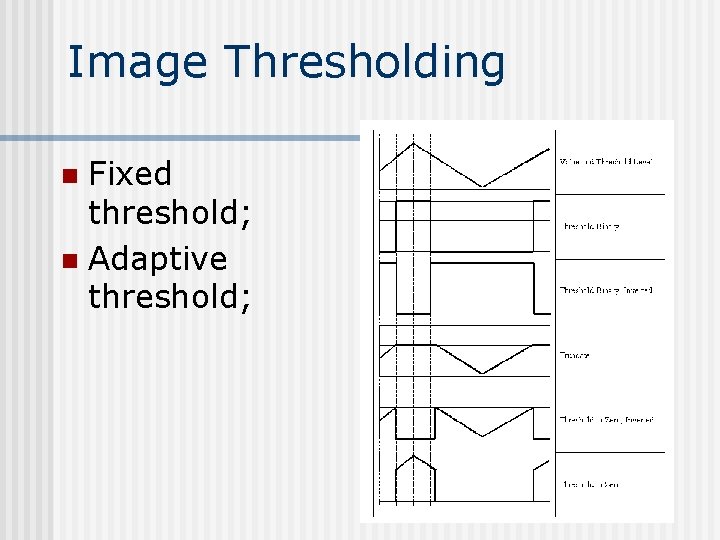
Image Thresholding Fixed threshold; n Adaptive threshold; n

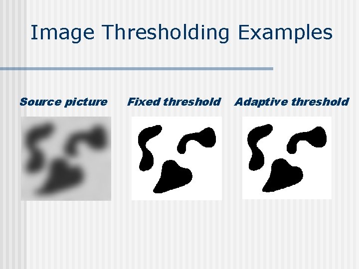
Image Thresholding Examples Source picture Fixed threshold Adaptive threshold

Victor Eruhimov: Statistics n n In addition to simple norm calculation, there is a function that finds the norm of the difference between two images. min, max, mean value, standard deviation over the image Norms C, L 1, L 2 Multidimensional histograms Spatial moments up to order 3 (central, normalized, Hu)

Multidimensional Histograms n n Histogram operations : calculation, normalization, comparison, back project Histograms types: ü ü n Dense histograms Signatures (balanced tree) EMD algorithm: n n n The EMD computes the distance between two distributions, which are represented by signatures. The signatures are sets of weighted features that capture the distributions. The features can be of any type and in any number of dimensions, and are defined by the user. The EMD is defined as the minimum amount of work needed to change one signature into the other

EMD – a method for the histograms comparison

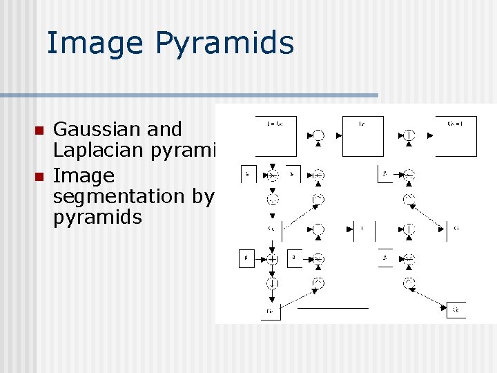
Image Pyramids n n Gaussian and Laplacian pyramids Image segmentation by pyramids

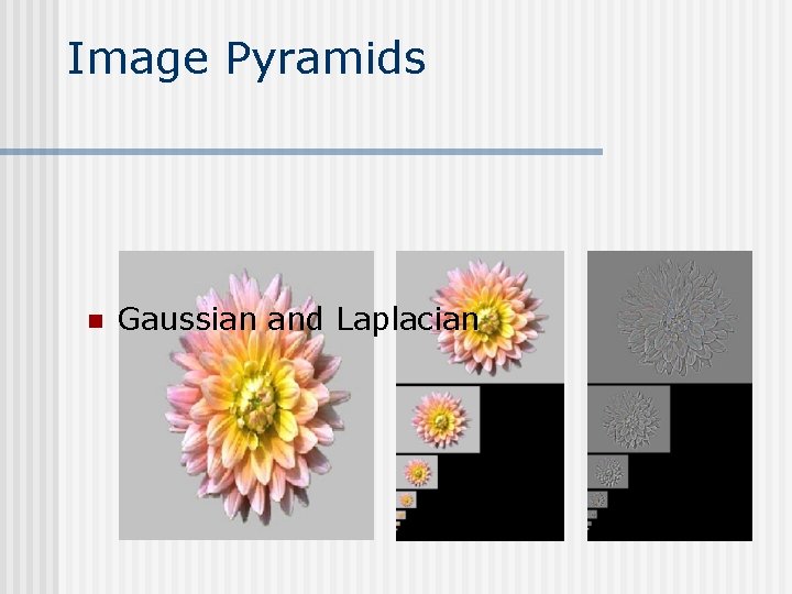
Image Pyramids n Gaussian and Laplacian

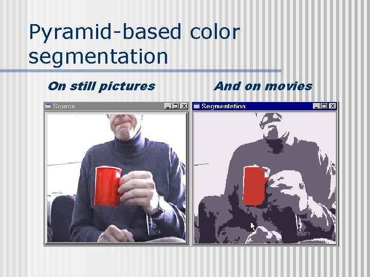
Pyramid-based color segmentation On still pictures And on movies

Morphological Operations n Two basic morphology operations using structuring element: ü erosion ü dilation n More complex morphology operations: ü ü ü opening closing morphological gradient top hat black hat

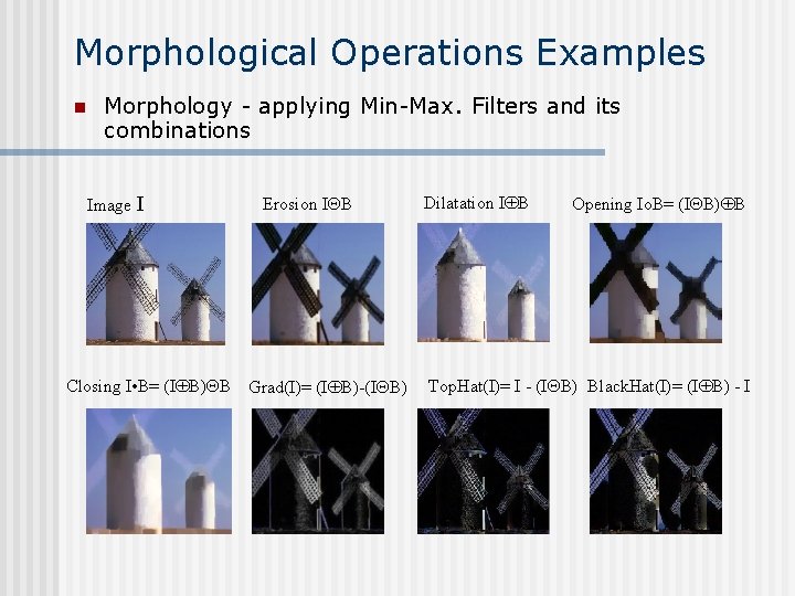
Morphological Operations Examples n Morphology - applying Min-Max. Filters and its combinations Image I Erosion I B Closing I • B= (I B) B Grad(I)= (I B)-(I B) Dilatation I B Opening Io. B= (I B) B Top. Hat(I)= I - (I B) Black. Hat(I)= (I B) - I

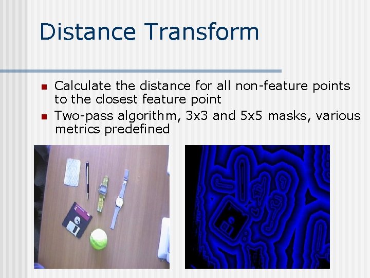
Distance Transform n n Calculate the distance for all non-feature points to the closest feature point Two-pass algorithm, 3 x 3 and 5 x 5 masks, various metrics predefined

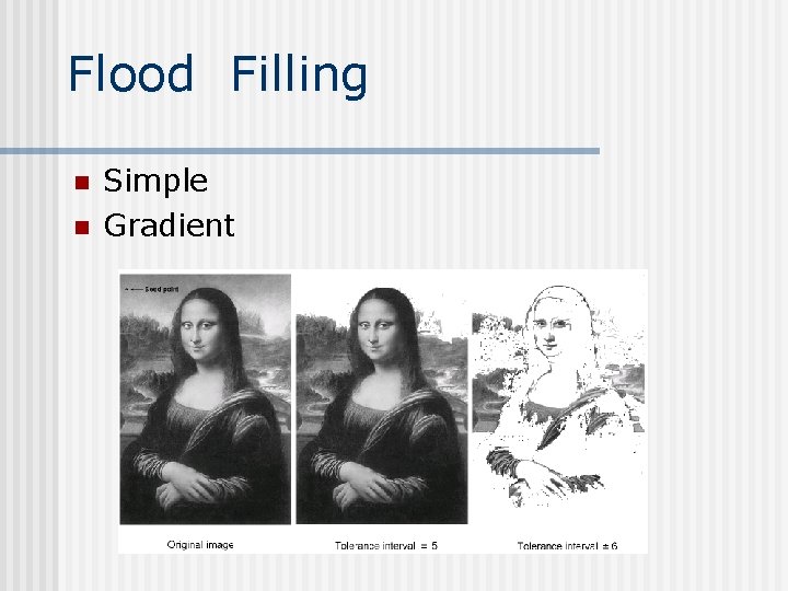
Flood Filling n n Simple Gradient

Feature Detection n n n Fixed filters (Sobel operator, Laplacian); Optimal filter kernels with floating point coefficients (first, second derivatives, Laplacian) Special feature detection (corners) Canny operator Hough transform (find lines and line segments) Gradient runs

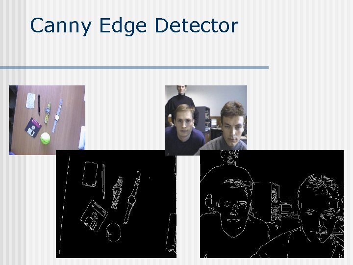
Canny Edge Detector

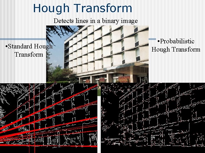
Hough Transform Detects lines in a binary image • Standard Hough Transform • Probabilistic Hough Transform

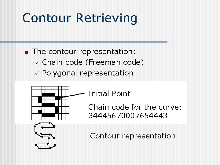
Contour Retrieving n The contour representation: ü Chain code (Freeman code) ü Polygonal representation Initial Point Chain code for the curve: 34445670007654443 Contour representation

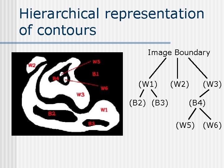
Hierarchical representation of contours Image Boundary (W 1) (B 2) (B 3) (W 2) (W 3) (B 4) (W 5) (W 6)

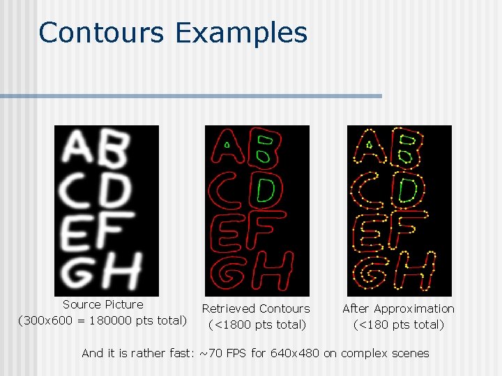
Contours Examples Source Picture (300 x 600 = 180000 pts total) Retrieved Contours (<1800 pts total) After Approximation (<180 pts total) And it is rather fast: ~70 FPS for 640 x 480 on complex scenes

Open. CV Functionality ü ü • n n n Basic structures and operations Image Analysis Structural Analysis Object Recognition Motion Analysis and Object Tracking 3 D Reconstruction

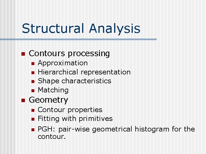
Structural Analysis n Contours processing n n n Approximation Hierarchical representation Shape characteristics Matching Geometry n n n Contour properties Fitting with primitives PGH: pair-wise geometrical histogram for the contour.

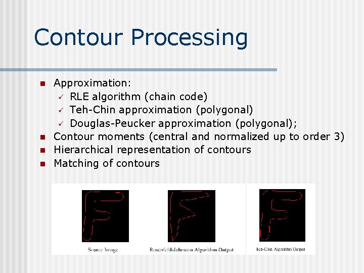
Contour Processing n n Approximation: ü RLE algorithm (chain code) ü Teh-Chin approximation (polygonal) ü Douglas-Peucker approximation (polygonal); Contour moments (central and normalized up to order 3) Hierarchical representation of contours Matching of contours

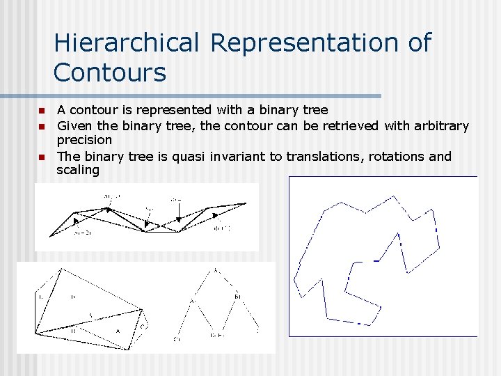
Hierarchical Representation of Contours n n n A contour is represented with a binary tree Given the binary tree, the contour can be retrieved with arbitrary precision The binary tree is quasi invariant to translations, rotations and scaling

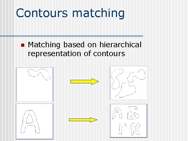
Contours matching n Matching based on hierarchical representation of contours

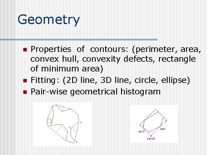
Geometry n n n Properties of contours: (perimeter, area, convex hull, convexity defects, rectangle of minimum area) Fitting: (2 D line, 3 D line, circle, ellipse) Pair-wise geometrical histogram

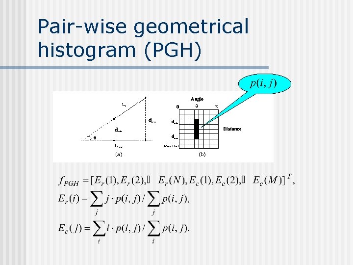
Pair-wise geometrical histogram (PGH)

Open. CV Functionality ü ü ü • n n Basic structures and operations Image Analysis Structural Analysis Object Recognition Motion Analysis and Object Tracking 3 D Reconstruction

Object Recognition Eigen objects n Hidden Markov Models n

Eigen Objects

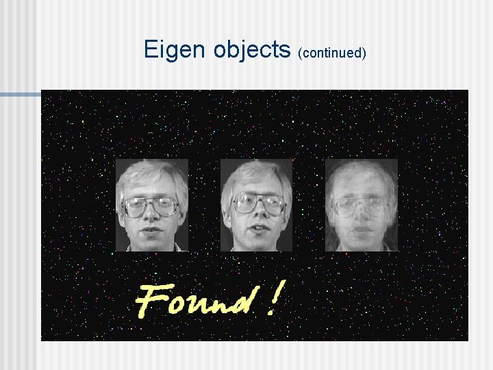
Eigen objects (continued)

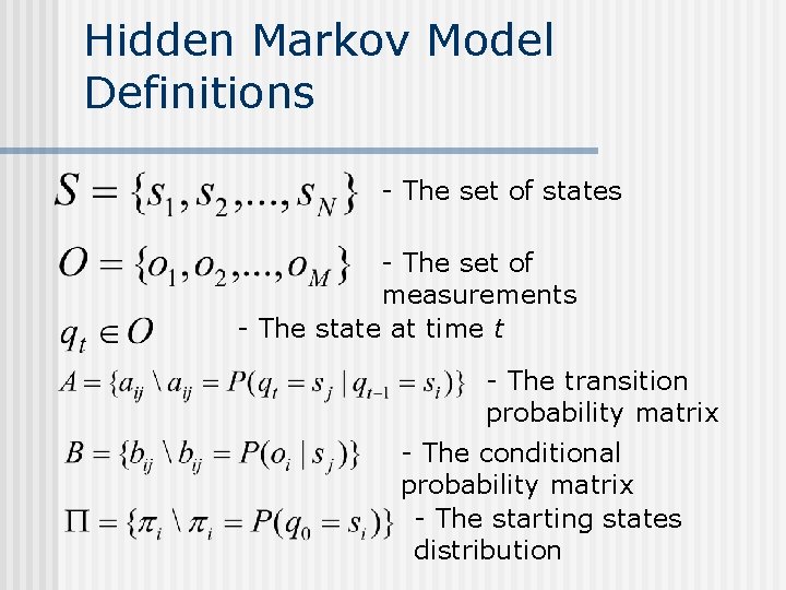
Hidden Markov Model Definitions - The set of states - The set of measurements - The state at time t - The transition probability matrix - The conditional probability matrix - The starting states distribution

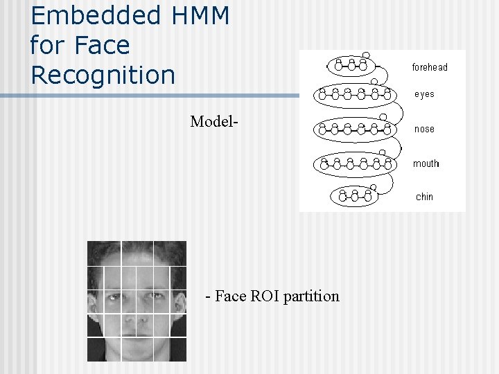
Embedded HMM for Face Recognition Model- - Face ROI partition

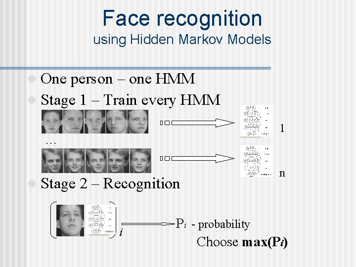
Face recognition using Hidden Markov Models l One person – one HMM l Stage 1 – Train every HMM 1 … l Stage 2 – Recognition i n Pi - probability Choose max(Pi)

Open. CV Functionality ü ü • n Basic structures and operations Image Analysis Structural Analysis Object Recognition Motion Analysis and Object Tracking 3 D Reconstruction

Motion Analysis and Object Tracking Background subtraction n Motion templates n Optical flow n Active contours n Estimators n

Background Subtraction Background model (normal distribution) n Background statistics functions: n Average ü Standard deviation ü Running average ü

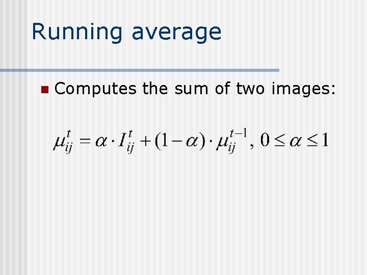
Running average n Computes the sum of two images:

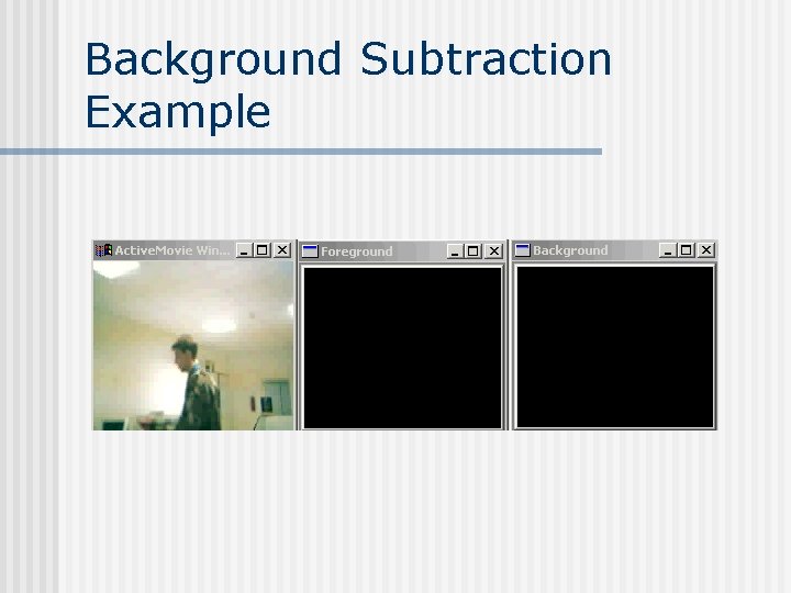
Background Subtraction Example

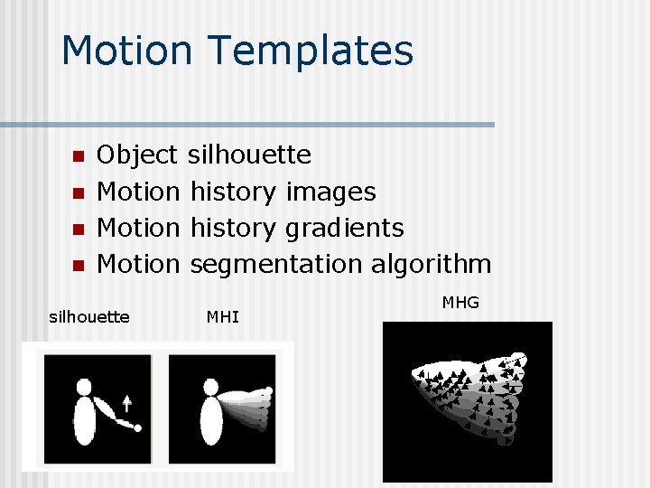
Motion Templates n n Object silhouette Motion history images Motion history gradients Motion segmentation algorithm silhouette MHI MHG

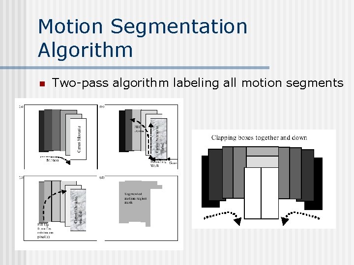
Motion Segmentation Algorithm n Two-pass algorithm labeling all motion segments

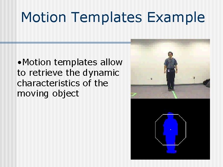
Motion Templates Example • Motion templates allow to retrieve the dynamic characteristics of the moving object

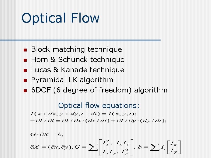
Optical Flow n n n Block matching technique Horn & Schunck technique Lucas & Kanade technique Pyramidal LK algorithm 6 DOF (6 degree of freedom) algorithm Optical flow equations:

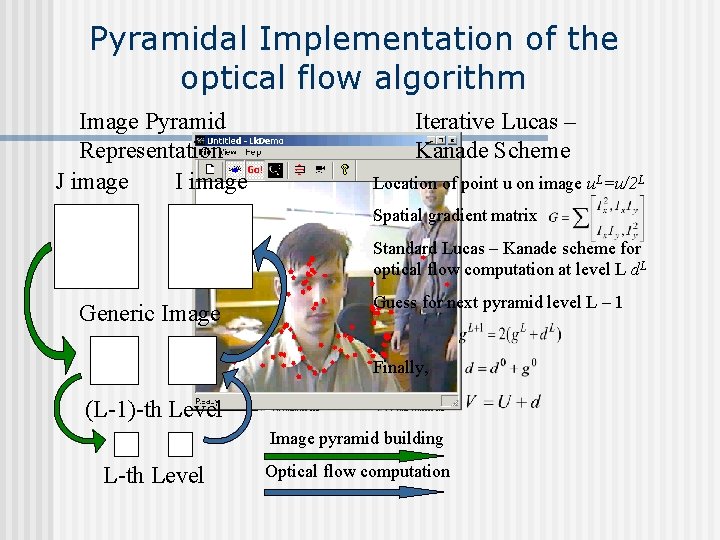
Pyramidal Implementation of the optical flow algorithm Image Pyramid Representation J image Iterative Lucas – Kanade Scheme Location of point u on image u. L=u/2 L Spatial gradient matrix Standard Lucas – Kanade scheme for optical flow computation at level L d. L Generic Image Guess for next pyramid level L – 1 Finally, (L-1)-th Level Image pyramid building L-th Level Optical flow computation

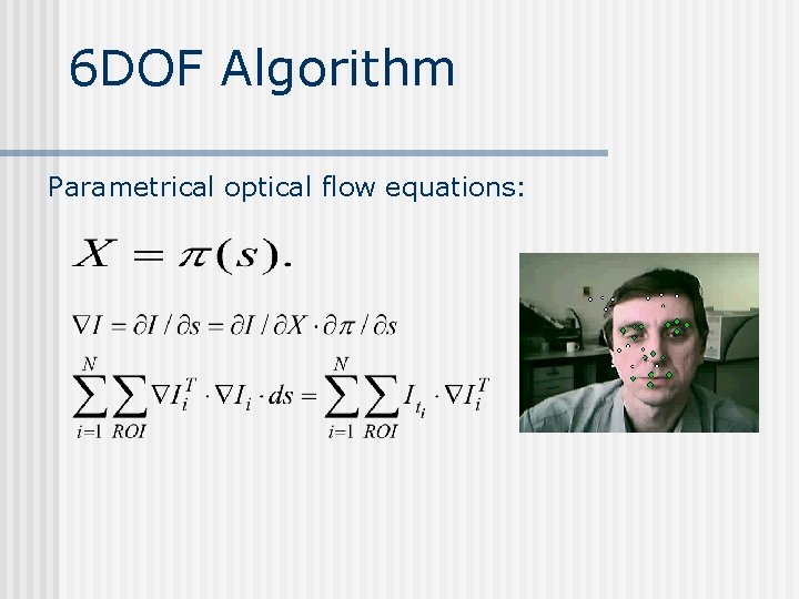
6 DOF Algorithm Parametrical optical flow equations:

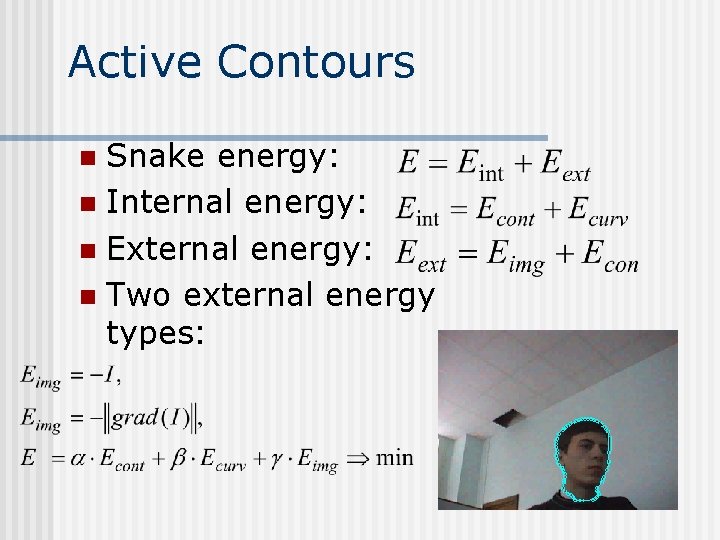
Active Contours Snake energy: n Internal energy: n External energy: n Two external energy types: n

Estimators n Kalman filter n Con. Densation filter

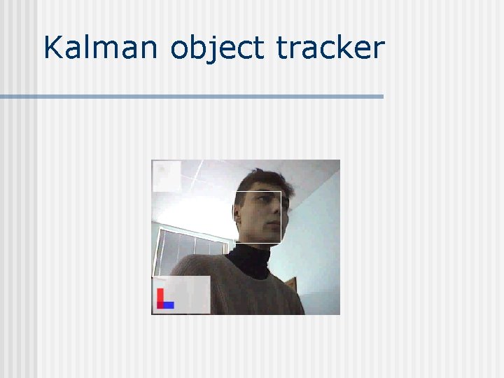
Kalman object tracker

Open. CV Functionality ü ü ü • Basic structures and operations Image Analysis Structural Analysis Object Recognition Motion Analysis and Object Tracking 3 D Reconstruction

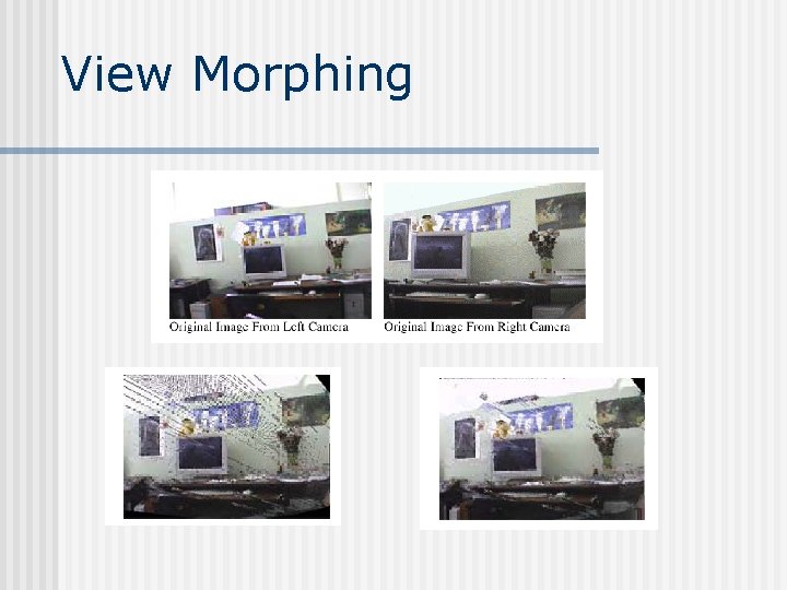
3 D reconstruction Camera Calibration n View Morphing n POSIT n

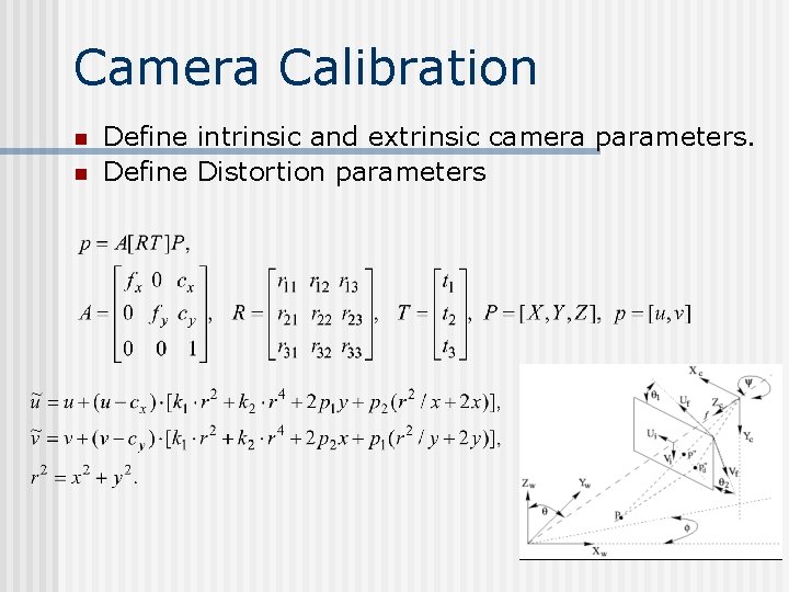
Camera Calibration n n Define intrinsic and extrinsic camera parameters. Define Distortion parameters

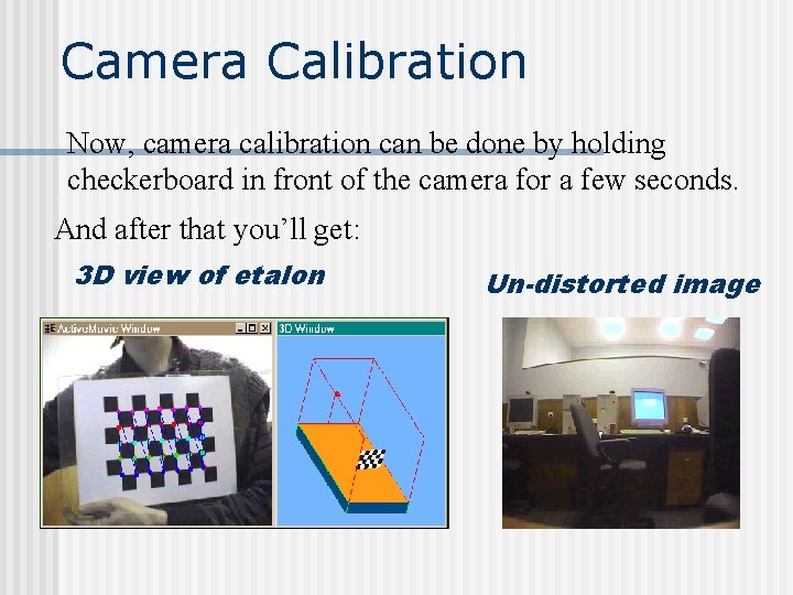
Camera Calibration Now, camera calibration can be done by holding checkerboard in front of the camera for a few seconds. And after that you’ll get: 3 D view of etalon Un-distorted image

View Morphing

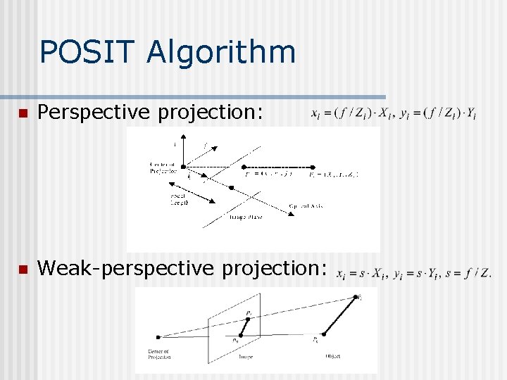
POSIT Algorithm n Perspective projection: n Weak-perspective projection:

Open. CV web sites n n http: //www. intel. com/research/mrl/research/opencv/ http: //sourceforge. net

References n n n n Gunilla Borgefors. Distance Transformations in Digital Images. Computer Vision, Graphics and Image Processing 34, 344 -371, (1986). G. Bradski and J. Davis. Motion Segmentation and Pose Recognition with Motion History Gradients. IEEE WACV'00, 2000. P. J. Burt, T. H. Hong, A. Rosenfeld. Segmentation and Estimation of Image Region Properties Through Cooperative Hierarchical Computation. IEEE Tran. On SMC, Vol. 11, N. 12, 1981, pp. 802 -809. J. Canny. A Computational Approach to Edge Detection, IEEE Trans. on Pattern Analysis and Machine Intelligence, 8(6), pp. 679 -698 (1986). J. Davis and Bobick. The Representation and Recognition of Action Using Temporal Templates. MIT Media Lab Technical Report 402, 1997. Daniel F. De. Menthon and Larry S. Davis. Model-Based Object Pose in 25 Lines of Code. In Proceedings of ECCV '92, pp. 335 -343, 1992. Andrew W. Fitzgibbon, R. B. Fisher. A Buyer’s Guide to Conic Fitting. Proc. 5 th British Machine Vision Conference, Birmingham, pp. 513 -522, 1995. Berthold K. P. Horn and Brian G. Schunck. Determining Optical Flow. Artificial Intelligence, 17, pp. 185 -203, 1981.

References n n n n M. Hu. Visual Pattern Recognition by Moment Invariants, IRE Transactions on Information Theory, 8: 2, pp. 179 -187, 1962. B. Jahne. Digital Image Processing. Springer, New York, 1997. M. Kass, A. Witkin, and D. Terzopoulos. Snakes: Active Contour Models, International Journal of Computer Vision, pp. 321 -331, 1988. J. Matas, C. Galambos, J. Kittler. Progressive Probabilistic Hough Transform. British Machine Vision Conference, 1998. A. Rosenfeld and E. Johnston. Angle Detection on Digital Curves. IEEE Trans. Computers, 22: 875 -878, 1973. Y. Rubner. C. Tomasi, L. J. Guibas. Metrics for Distributions with Applications to Image Databases. Proceedings of the 1998 IEEE International Conference on Computer Vision, Bombay, India, January 1998, pp. 59 -66. Y. Rubner. C. Tomasi, L. J. Guibas. The Earth Mover’s Distance as a Metric for Image Retrieval. Technical Report STAN-CS-TN-98 -86, Department of Computer Science, Stanford University, September, 1998. Y. Rubner. C. Tomasi. Texture Metrics. Proceeding of the IEEE International Conference on Systems, Man, and Cybernetics, San-Diego, CA, October 1998, pp. 4601 - 4607. http: //robotics. stanford. edu/~rubner/publications. html

References n n n n J. Serra. Image Analysis and Mathematical Morphology. Academic Press, 1982. Bernt Schiele and James L. Crowley. Recognition without Correspondence Using Multidimensional Receptive Field Histograms. In International Journal of Computer Vision 36 (1), pp. 31 -50, January 2000. S. Suzuki, K. Abe. Topological Structural Analysis of Digital Binary Images by Border Following. CVGIP, v. 30, n. 1. 1985, pp. 32 -46. C. H. Teh, R. T. Chin. On the Detection of Dominant Points on Digital Curves. - IEEE Tr. PAMI, 1989, v. 11, No. 8, p. 859 -872. Emanuele Trucco, Alessandro Verri. Introductory Techniques for 3 -D Computer Vision. Prentice Hall, Inc. , 1998. D. J. Williams and M. Shah. A Fast Algorithm for Active Contours and Curvature Estimation. CVGIP: Image Understanding, Vol. 55, No. 1, pp. 14 -26, Jan. , 1992. http: //www. cs. ucf. edu/~vision/papers/shah/92/WIS 92 A. pdf. A. Y. Yuille, D. S. Cohen, and P. W. Hallinan. Feature Extraction from Faces Using Deformable Templates in CVPR, pp. 104 -109, 1989. Zhengyou Zhang. Parameter Estimation Techniques: A Tutorial with Application to Conic Fitting, Image and Vision Computing Journal, 1996.

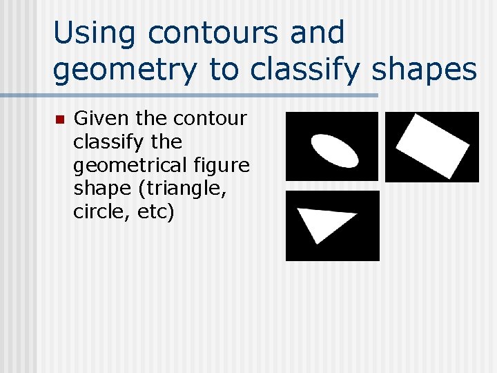
Using contours and geometry to classify shapes n Given the contour classify the geometrical figure shape (triangle, circle, etc)

Open. CV shape classification capabilities n Contour approximation n Moments (image&contour) n Convexity analysis n Pair-wise geometrical histogram n Fitting functions (line, ellipse)

Contour approximation n Min-epsilon approximation (Imai&Iri) n Min#-approximation (Douglas. Peucker method) Hawk

Moments n Image moments (binary, grayscale) n Contour moments (faster) n Hu invariants

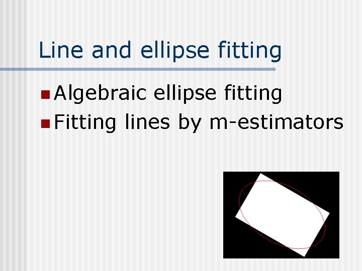
Line and ellipse fitting n Algebraic ellipse fitting n Fitting lines by m-estimators

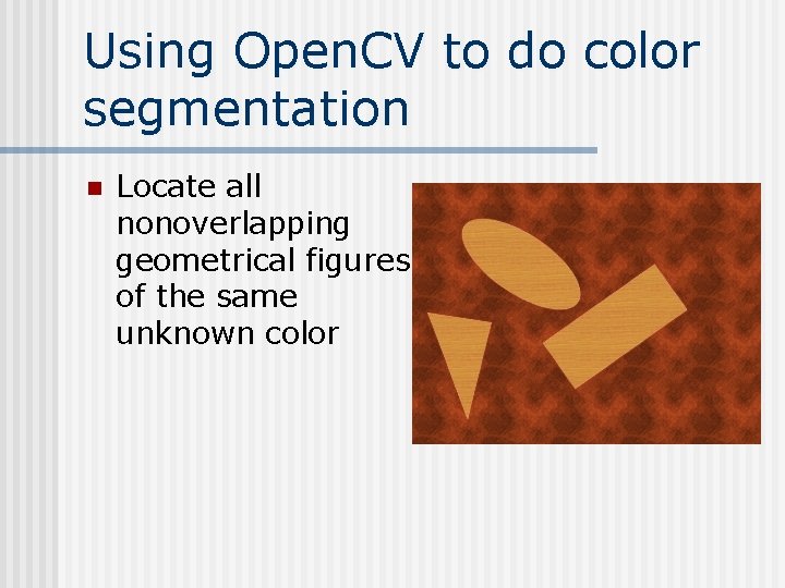
Using Open. CV to do color segmentation n Locate all nonoverlapping geometrical figures of the same unknown color

Open. CV segmentation capabilities n Edge-based approach n Histogram n Color segmentation

Edge-based segmentation Smoothing functions (gaussian filter. IPL, bilateral filter) n Apply edge detector (sobel, laplace, canny, gradient strokes) n Find connected components in an inverted image n

Pyramid segmentation n Water down the color space in order to join up the neighbor image pixels that are close to each other in XY and color spaces Call Hawk here

Histogram Calculate the histogram n Separate the object and background histograms n Find the objects of the selected histogram in the image n Call Hawk here

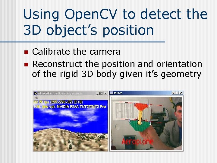
Using Open. CV to detect the 3 D object’s position n n Calibrate the camera Reconstruct the position and orientation of the rigid 3 D body given it’s geometry

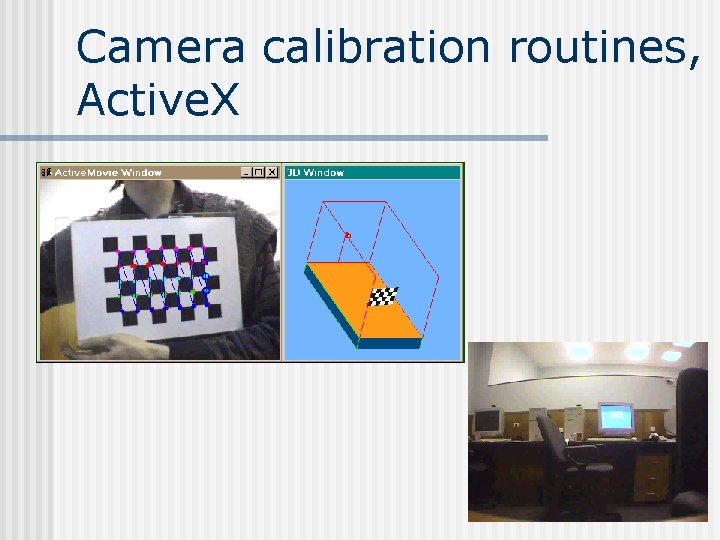
Camera calibration routines, Active. X

Reconstruction task Given n camera model 3 D coordinates of the feature points and 2 D coordinates corresponding projections on the image Reconstruct the 3 D position and orientation

Reconstruction task (continued) POSIT algorithm for 3 D objects n Find. Extrinsic. Camera. Params for arbitrary objects n

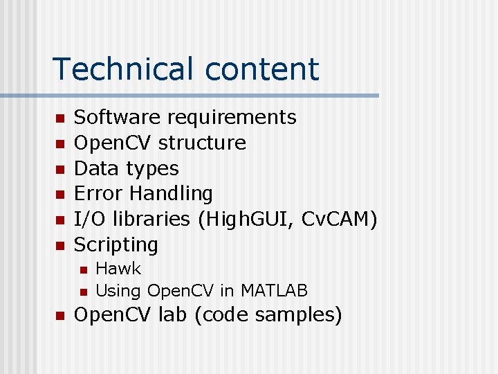
Technical content n n n Software requirements Open. CV structure Data types Error Handling I/O libraries (High. GUI, Cv. CAM) Scripting n n n Hawk Using Open. CV in MATLAB Open. CV lab (code samples)

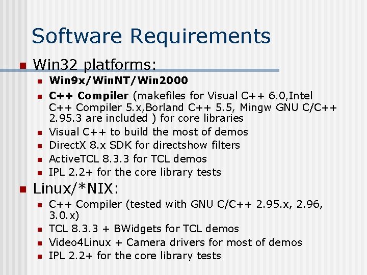
Software Requirements n Win 32 platforms: n Win 9 x/Win. NT/Win 2000 n C++ Compiler (makefiles for Visual C++ 6. 0, Intel C++ Compiler 5. x, Borland C++ 5. 5, Mingw GNU C/C++ 2. 95. 3 are included ) for core libraries Visual C++ to build the most of demos Direct. X 8. x SDK for directshow filters Active. TCL 8. 3. 3 for TCL demos IPL 2. 2+ for the core library tests n n n Linux/*NIX: n n C++ Compiler (tested with GNU C/C++ 2. 95. x, 2. 96, 3. 0. x) TCL 8. 3. 3 + BWidgets for TCL demos Video 4 Linux + Camera drivers for most of demos IPL 2. 2+ for the core library tests

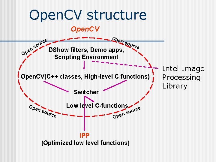
Open. CV structure Open. CV e Op ou ns Ope rce n so DShow filters, Demo apps, Scripting Environment urc e Open. CV(C++ classes, High-level C functions) Switcher Ope n so urc e Low level C-functions rce u o ns e p O IPP (Optimized low level functions) Intel Image Processing Library

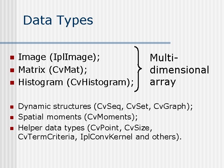
Data Types n n n Image (Ipl. Image); Matrix (Cv. Mat); Histogram (Cv. Histogram); Multidimensional array Dynamic structures (Cv. Seq, Cv. Set, Cv. Graph); Spatial moments (Cv. Moments); Helper data types (Cv. Point, Cv. Size, Cv. Term. Criteria, Ipl. Conv. Kernel and others).

Error Handling There are no return error codes n There is a global error status that can be set or checked via special functions n By default a message box appears if error happens n

Portable GUI library (High. GUI) n n n Reading/Writing images in several formats (BMP, JPEG, TIFF, Px. M, Sun Raster) Creating windows and displaying images in it. High. GUI windows remember their content (no need to implement repainting callbacks) Simple interaction facilities: trackbars, getting input from keyboard and mouse (new in Win 32 version).

Portable Video Capture Library (Cv. CAM) n n n Single interface for video capture and playback under Linux and Win 32 Provides callback for subsequent processing of frames from camera or AVI-file Easy stereo from 2 USB cameras or stereo-camera

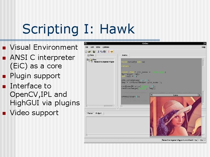
Scripting I: Hawk n n n Visual Environment ANSI C interpreter (Ei. C) as a core Plugin support Interface to Open. CV, IPL and High. GUI via plugins Video support

Scripting II: Open. CV + MATLAB Design principles and data types organization n Working with images n Working with dynamic structures n Example n

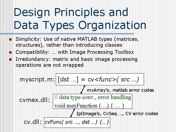
Design Principles and Data Types Organization n Simplicity: Use of native MATLAB types (matrices, structures), rather than introducing classes Compatibility: … with Image Processing Toolbox Irredundancy: matrix and basic image processing operations are not wrapped myscript. m: [dst …] = cv<func>( src …) mx. Array’s, matlab error codes cvmex. dll: // data type conv. , error handling void mex. Function (…) { … } Ipl. Image’s, Cv. Seq …, CV error codes cv. dll: cv. Func( src …, dst …) {…}

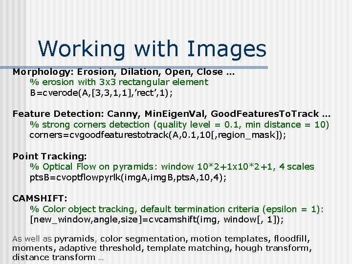
Working with Images Morphology: Erosion, Dilation, Open, Close … % erosion with 3 x 3 rectangular element B=cverode(A, [3, 3, 1, 1], ’rect’, 1); Feature Detection: Canny, Min. Eigen. Val, Good. Features. To. Track … % strong corners detection (quality level = 0. 1, min distance = 10) corners=cvgoodfeaturestotrack(A, 0. 1, 10[, region_mask]); Point Tracking: % Optical Flow on pyramids: window 10*2+1 x 10*2+1, 4 scales pts. B=cvoptflowpyrlk(img. A, img. B, pts. A, 10, 4); CAMSHIFT: % Color object tracking, default termination criteria (epsilon = 1): [new_window, angle, size]=cvcamshift(img, window[, 1]); As well as pyramids, color segmentation, motion templates, floodfill, moments, adaptive threshold, template matching, hough transform, distance transform …

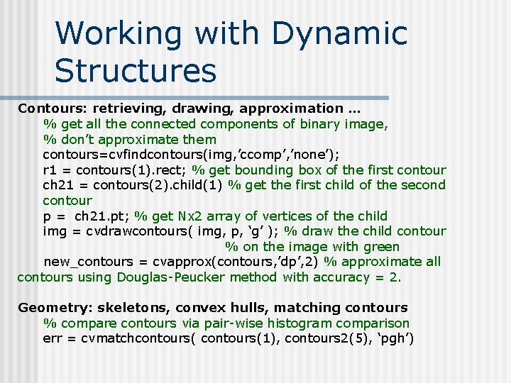
Working with Dynamic Structures Contours: retrieving, drawing, approximation … % get all the connected components of binary image, % don’t approximate them contours=cvfindcontours(img, ’ccomp’, ’none’); r 1 = contours(1). rect; % get bounding box of the first contour ch 21 = contours(2). child(1) % get the first child of the second contour p = ch 21. pt; % get Nx 2 array of vertices of the child img = cvdrawcontours( img, p, ‘g’ ); % draw the child contour % on the image with green new_contours = cvapprox(contours, ’dp’, 2) % approximate all contours using Douglas-Peucker method with accuracy = 2. Geometry: skeletons, convex hulls, matching contours % compare contours via pair-wise histogram comparison err = cvmatchcontours(1), contours 2(5), ‘pgh’)

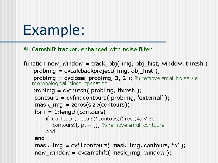
Example: % Camshift tracker, enhanced with noise filter function new_window = track_obj( img, obj_hist, window, thresh ) probimg = cvcalcbackproject( img, obj_hist ); probimg = cvclose( probimg, 3, 2 ); % remove small holes via morphological ‘close’ operation probimg = cvthresh( probimg, thresh ); contours = cvfindcontours( probimg, ‘external’ ); mask_img = zeros(size(contours)); for i = 1: length(contours) if contous(i). rect(3)*contous(i). rect(4) < 30 contours(i). pt = []; % remove small contours; end mask_img = cvfillcontours( mask_img, contours, ‘w’ ); new_window = cvcamshift( mask_img, window );

Victor Eruhimov: Questions?

Trainings Go to lab…