Integer programming Group members Ibrahim jan Qesar Habib

Integer programming Group members: Ibrahim jan Qesar Habib Najeebullah

Linear programming �Linear programming (LP, or linear optimization) is a mathematical method. � for determining a way to achieve the best outcome (such as maximum profit or lowest cost). �mathematical model for some list of requirements represented as linear relationships. � Linear programming is a specific case of mathematical programming (mathematical optimization).

�More formally, linear programming is a technique for the optimization of a linear objective function, subject to linear equality and linear inequality constraints.

Integer linear programming �An integer programming problem is a mathematical optimization or feasibility program in which some or all of the variables are restricted to be integers. �Integer programming problem are a special class of linear programming where all are some of the variable in the optimal solution are restricted to non-negative integer value.

�Linear programming problem are based on assumption that the decision variable are continuous with the result that they may take frictional value in the optimal solution e. g. 143/5 unit of product. �However many situation in real life may not allow for this and warrant for the decision variable to take only integer value.

�For example in production, manufacturing is frequently scheduled in term of lots, batches or production runs. �In allocation of goods, a shipment of goods involve discrete number of trucks, wagon or aircraft and fractional values are meaningless.

Types of integers �Pure and mixed integer programming. (1) An integer programming in which all variable are required to be integer is called pure integer. (2) An integer programming in which some variable are required to be integer is called mixed integer programming.

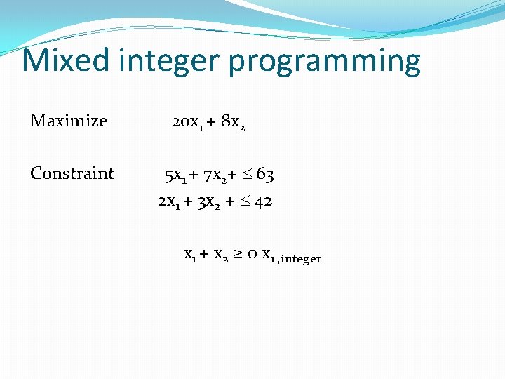
Mixed integer programming Maximize Constraint 20 x 1 + 8 x 2 5 x 1 + 7 x 2+ 63 2 x 1 + 3 x 2 + 42 x 1 + x 2 ≥ 0 x 1 , integer

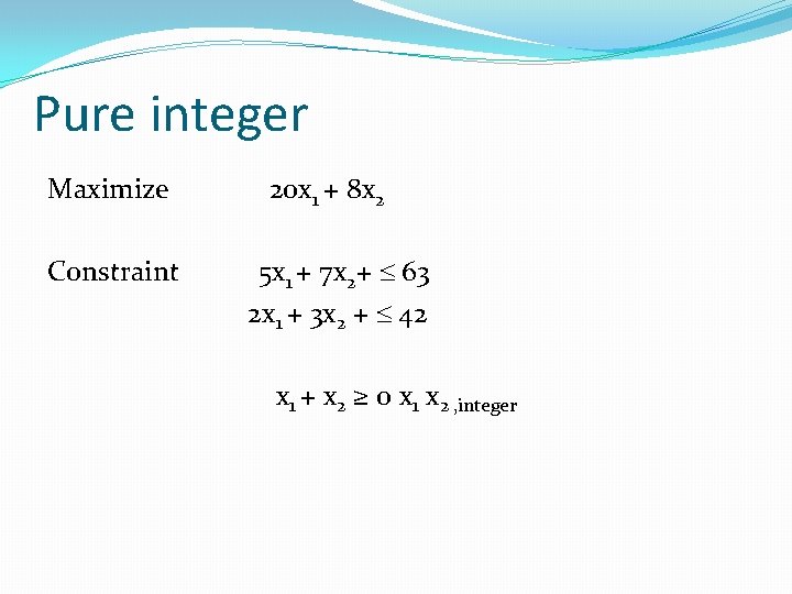
Pure integer Maximize Constraint 20 x 1 + 8 x 2 5 x 1 + 7 x 2+ 63 2 x 1 + 3 x 2 + 42 x 1 + x 2 ≥ 0 x 1 x 2 , integer

Zero-one Model Integer programming �A special type of integer programming problem is a case where the value of decision variable are limited to logical variable like Yes or No, Matched or No. Matched which are symbolized by the value 0 and 1

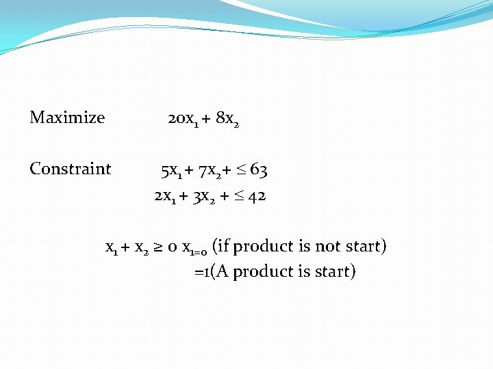
Maximize Constraint 20 x 1 + 8 x 2 5 x 1 + 7 x 2+ 63 2 x 1 + 3 x 2 + 42 x 1 + x 2 ≥ 0 x 1=0 (if product is not start) =1(A product is start)

Applications of integer programming �Integer program is used in following. 1. Traveling sales man problem. 2. Capital budgeting. 3. Facility location. 4. Fixed charge problem.

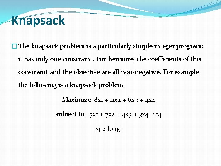
Knapsack �The knapsack problem is a particularly simple integer program: it has only one constraint. Furthermore, the coefficients of this constraint and the objective are all non-negative. For example, the following is a knapsack problem: Maximize 8 x 1 + 11 x 2 + 6 x 3 + 4 x 4 subject to 5 x 1 + 7 x 2 + 4 x 3 + 3 x 4 ≤ 14 xj 2 f 0; 1 g:

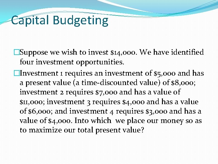
Capital Budgeting �Suppose we wish to invest $14, 000. We have identified four investment opportunities. �Investment 1 requires an investment of $5, 000 and has a present value (a time-discounted value) of $8, 000; investment 2 requires $7, 000 and has a value of $11, 000; investment 3 requires $4, 000 and has a value of $6, 000; and investment 4 requires $3, 000 and has a value of $4, 000. Into which we place our money so as to maximize our total present value?

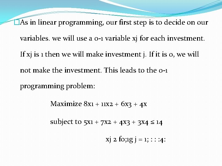
�As in linear programming, our first step is to decide on our variables. we will use a 0 -1 variable xj for each investment. If xj is 1 then we will make investment j. If it is 0, we will not make the investment. This leads to the 0 -1 programming problem: Maximize 8 x 1 + 11 x 2 + 6 x 3 + 4 x subject to 5 x 1 + 7 x 2 + 4 x 3 + 3 x 4 ≤ 14 xj 2 f 0; 1 g j = 1; : : : 4:

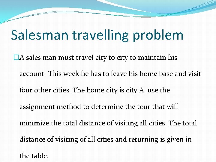
Salesman travelling problem �A sales man must travel city to maintain his account. This week he has to leave his home base and visit four other cities. The home city is city A. use the assignment method to determine the tour that will minimize the total distance of visiting all cities. The total distance of visiting of all cities and returning is given in the table.

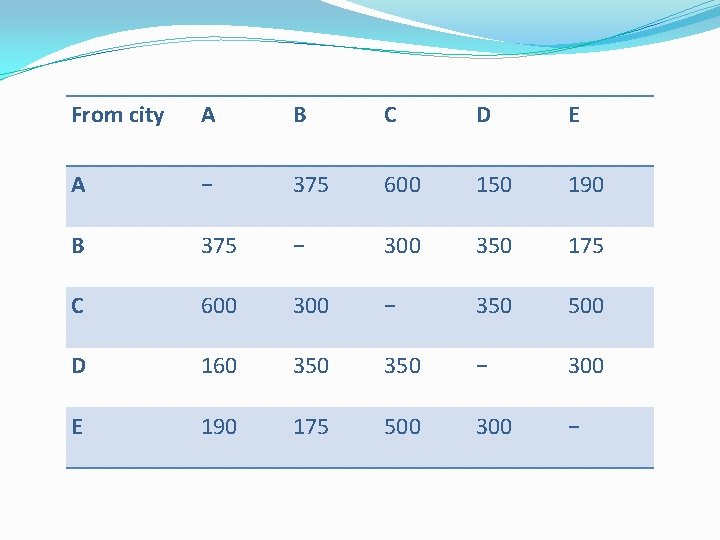
From city A B C D E A − 375 600 150 190 B 375 − 300 350 175 C 600 300 − 350 500 D 160 350 − 300 E 190 175 500 300 −

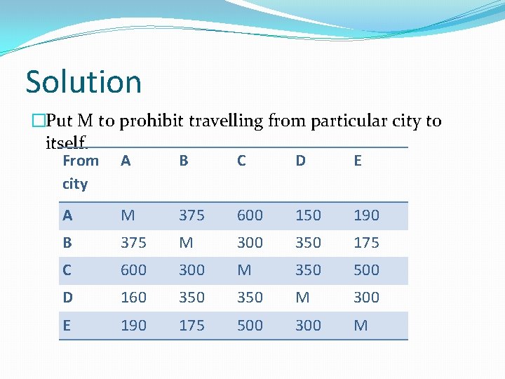
Solution �Put M to prohibit travelling from particular city to itself. From A B C D E city A M 375 600 150 190 B 375 M 300 350 175 C 600 300 M 350 500 D 160 350 M 300 E 190 175 500 300 M

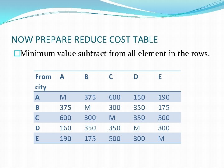
NOW PREPARE REDUCE COST TABLE �Minimum value subtract from all element in the rows. From city A B C D E M 375 600 160 190 375 M 300 350 175 600 300 M 350 500 150 350 M 300 190 175 500 300 M

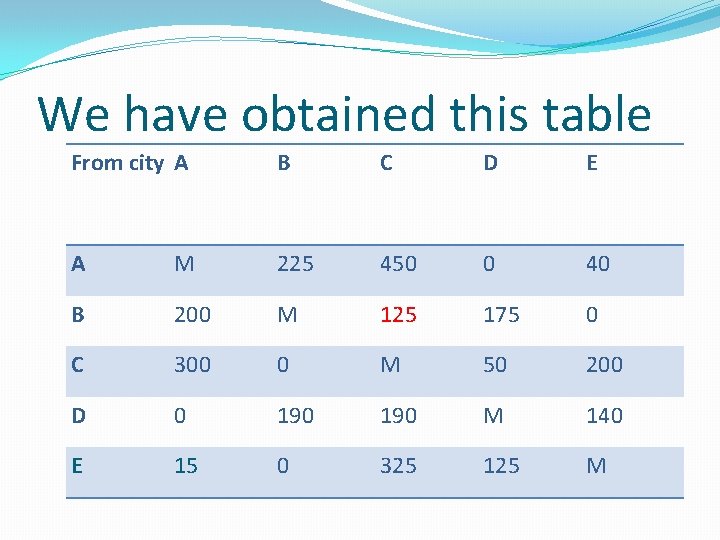
We have obtained this table From city A B C D E A M 225 450 0 40 B 200 M 125 175 0 C 300 0 M 50 200 D 0 190 M 140 E 15 0 325 125 M

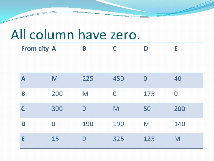
All column have zero. From city A B C D E A M 225 450 0 40 B 200 M 0 175 0 C 300 0 M 50 200 D 0 190 M 140 E 15 0 325 125 M

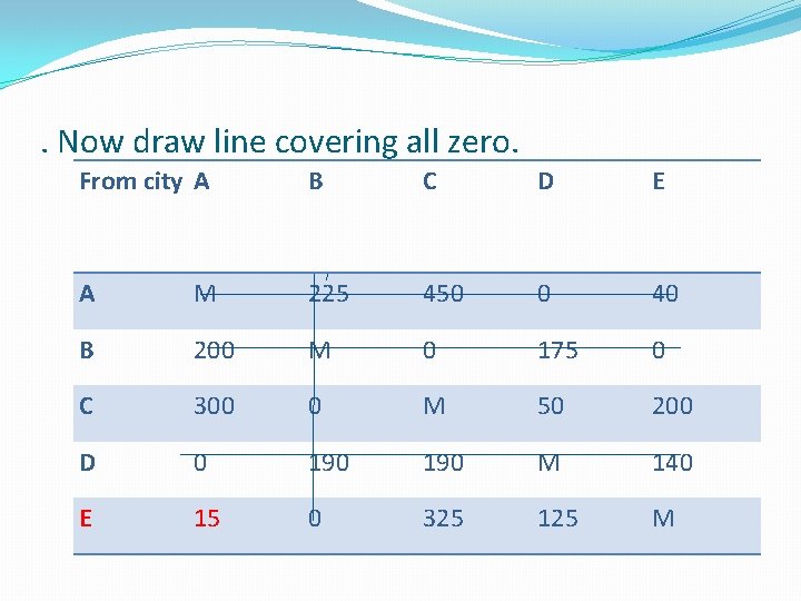
. Now draw line covering all zero. From city A B C D E A M 225 450 0 40 B 200 M 0 175 0 C 300 0 M 50 200 D 0 190 M 140 E 15 0 325 125 M

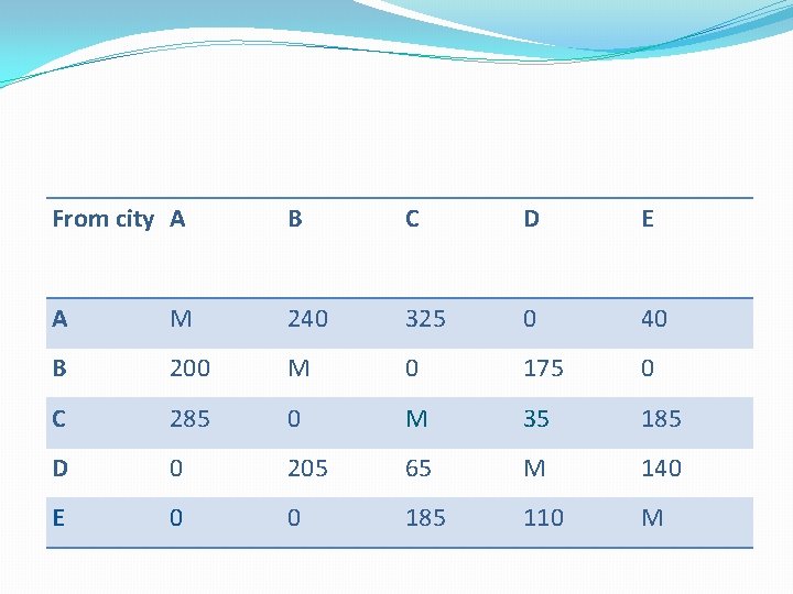
From city A B C D E A M 240 325 0 40 B 200 M 0 175 0 C 285 0 M 35 185 D 0 205 65 M 140 E 0 0 185 110 M

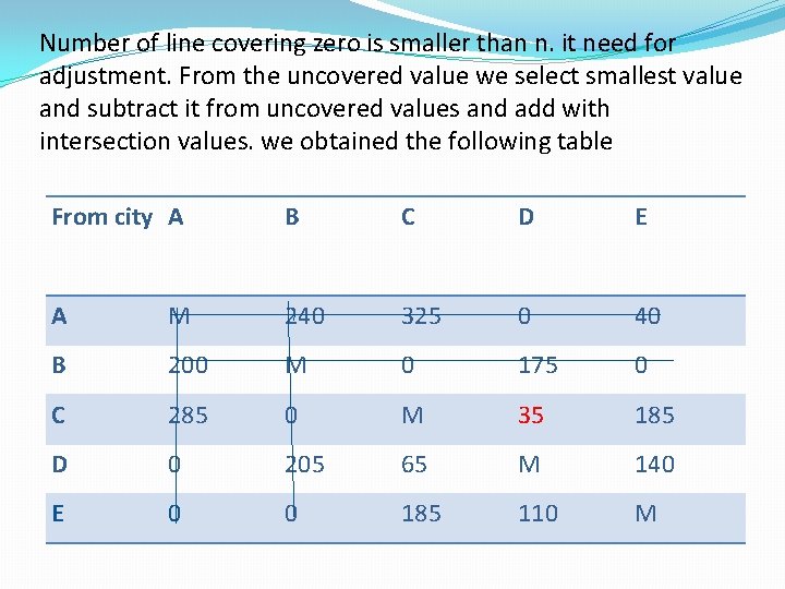
Number of line covering zero is smaller than n. it need for adjustment. From the uncovered value we select smallest value and subtract it from uncovered values and add with intersection values. we obtained the following table From city A B C D E A M 240 325 0 40 B 200 M 0 175 0 C 285 0 M 35 185 D 0 205 65 M 140 E 0 0 185 110 M

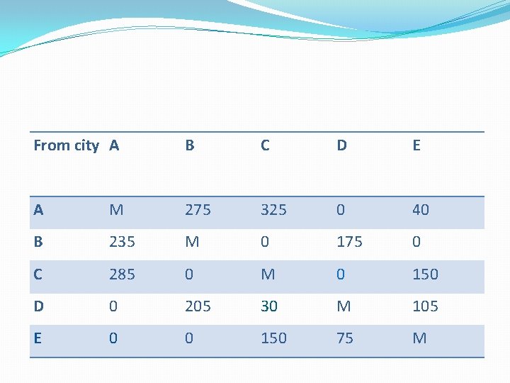
From city A B C D E A M 275 325 0 40 B 235 M 0 175 0 C 285 0 M 0 150 D 0 205 30 M 105 E 0 0 150 75 M

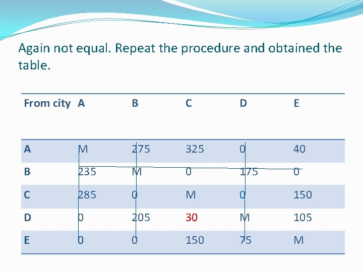
Again not equal. Repeat the procedure and obtained the table. From city A B C D E A M 275 325 0 40 B 235 M 0 175 0 C 285 0 M 0 150 D 0 205 30 M 105 E 0 0 150 75 M

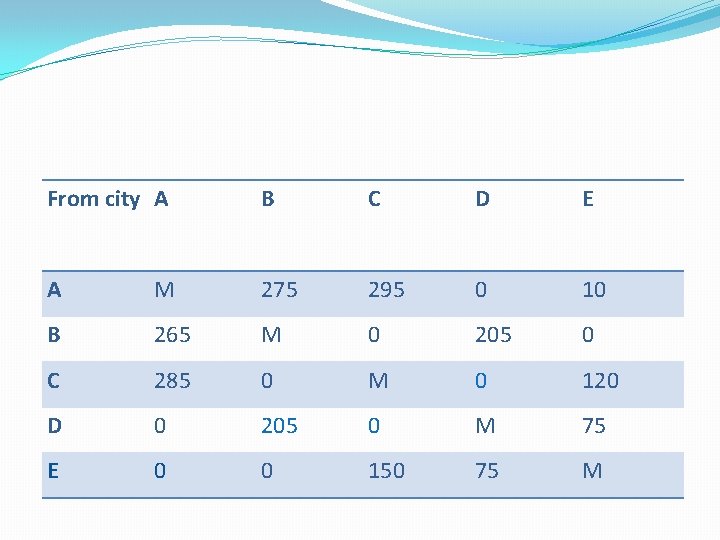
From city A B C D E A M 275 295 0 10 B 265 M 0 205 0 C 285 0 M 0 120 D 0 205 0 M 75 E 0 0 150 75 M

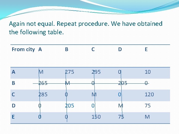
Again not equal. Repeat procedure. We have obtained the following table. From city A B C D E A M 275 295 0 10 B 265 M 0 205 0 C 285 0 M 0 120 D 0 205 0 M 75 E 0 0 150 75 M

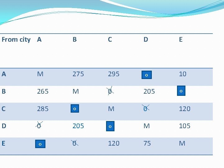
From city A B C D E A M 275 295 00 10 B 265 M 0 205 00 C 285 00 M 0 120 D 0 205 00 M 105 E 00 0 120 75 M

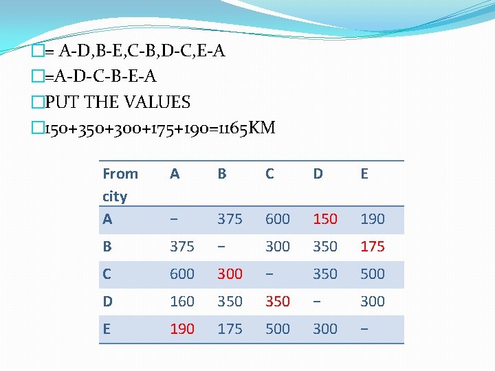
�= A-D, B-E, C-B, D-C, E-A �=A-D-C-B-E-A �PUT THE VALUES � 150+300+175+190=1165 KM From city A A B C D E − 375 600 150 190 B 375 − 300 350 175 C 600 300 − 350 500 D 160 350 − 300 E 190 175 500 300 −

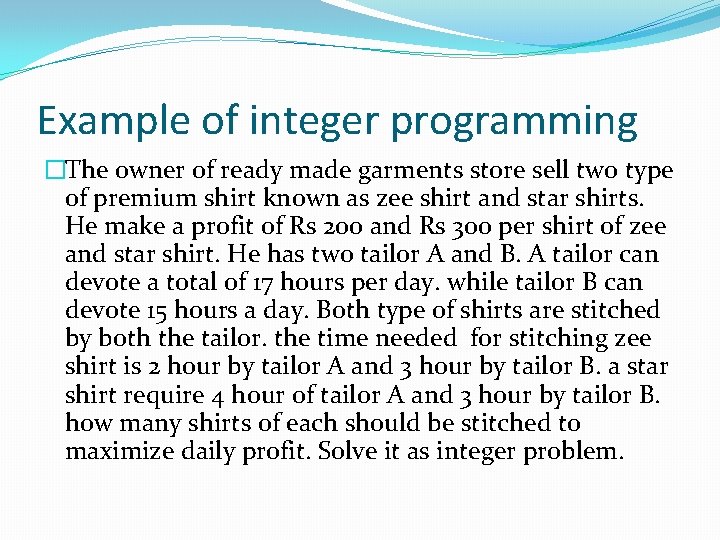
Example of integer programming �The owner of ready made garments store sell two type of premium shirt known as zee shirt and star shirts. He make a profit of Rs 200 and Rs 300 per shirt of zee and star shirt. He has two tailor A and B. A tailor can devote a total of 17 hours per day. while tailor B can devote 15 hours a day. Both type of shirts are stitched by both the tailor. the time needed for stitching zee shirt is 2 hour by tailor A and 3 hour by tailor B. a star shirt require 4 hour of tailor A and 3 hour by tailor B. how many shirts of each should be stitched to maximize daily profit. Solve it as integer problem.

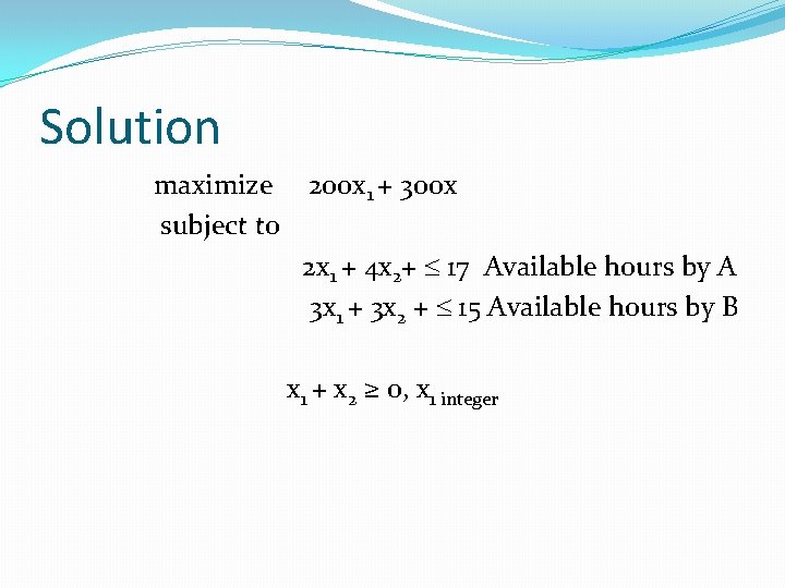
Solution maximize 2 oox 1 + 300 x subject to 2 x 1 + 4 x 2+ 17 Available hours by A 3 x 1 + 3 x 2 + 15 Available hours by B x 1 + x 2 ≥ 0, x 1 integer

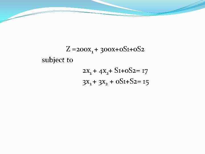
Z =2 oox 1 + 300 x+0 S 1+0 S 2 subject to 2 x 1 + 4 x 2+ S 1+0 S 2= 17 3 x 1 + 3 x 2 + 0 S 1+S 2= 15

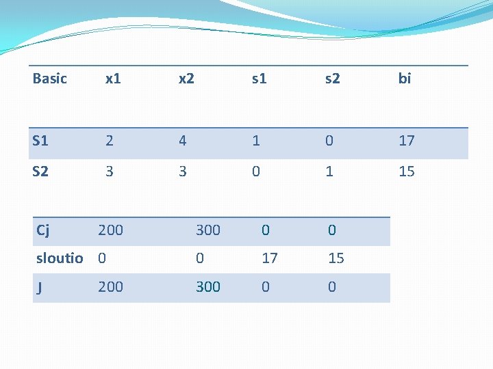
Basic x 1 x 2 s 1 s 2 bi S 1 2 4 1 0 17 S 2 3 3 0 1 15 Cj 200 sloutio 0 J 200 300 0 17 15 300 0 0

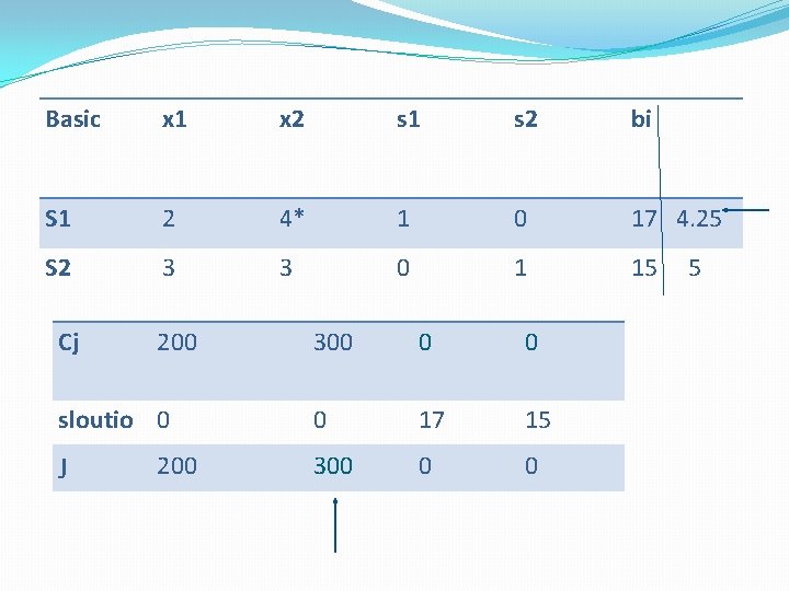
Basic x 1 x 2 s 1 s 2 bi S 1 2 4* 1 0 17 4. 25 S 2 3 3 0 1 15 Cj 200 sloutio 0 J 200 300 0 17 15 300 0 0 5

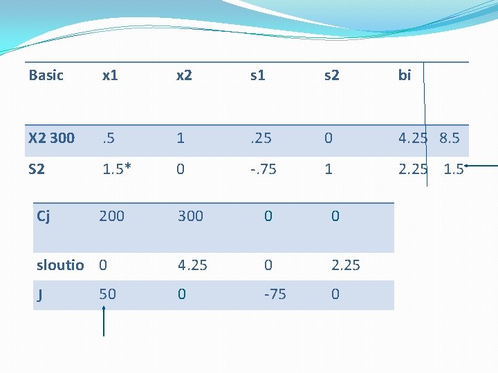
Basic x 1 x 2 s 1 s 2 bi X 2 300 . 5 1 . 25 0 4. 25 8. 5 S 2 1. 5* 0 -. 75 1 2. 25 1. 5 200 300 0 0 4. 25 0 2. 25 0 -75 0 Cj sloutio 0 J 50

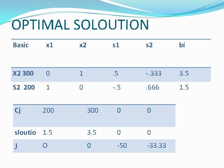
OPTIMAL SOLOUTION Basic x 1 x 2 s 1 s 2 bi X 2 300 0 1 . 5 -. 333 3. 5 S 2 200 1 0 -. 5 . 666 1. 5 Cj 200 300 0 0 sloutio 1. 5 3. 5 0 0 0 -50 -33. 33 J O

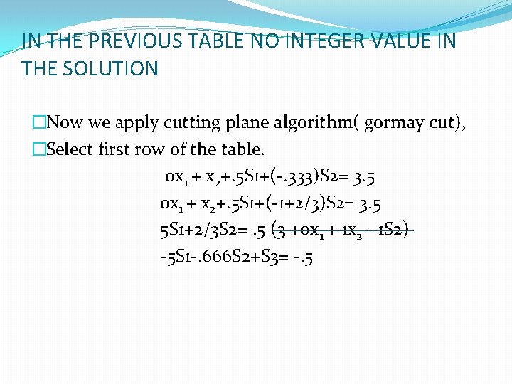
IN THE PREVIOUS TABLE NO INTEGER VALUE IN THE SOLUTION �Now we apply cutting plane algorithm( gormay cut), �Select first row of the table. 0 x 1 + x 2+. 5 S 1+(-. 333)S 2= 3. 5 0 x 1 + x 2+. 5 S 1+(-1+2/3)S 2= 3. 5 5 S 1+2/3 S 2=. 5 (3 +0 x 1 + 1 x 2 - 1 S 2) -5 S 1 -. 666 S 2+S 3= -. 5

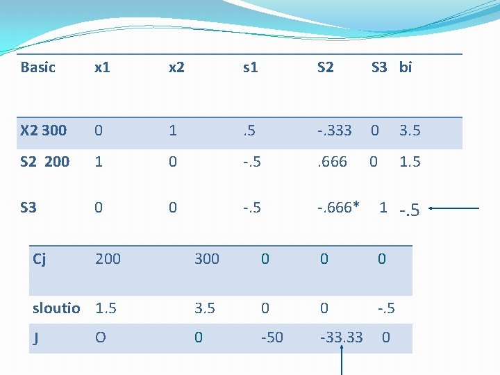
Basic x 1 x 2 s 1 S 2 S 3 bi X 2 300 0 1 . 5 -. 333 0 3. 5 S 2 200 1 0 -. 5 . 666 0 1. 5 S 3 0 0 -. 5 -. 666* 1 -. 5 Cj 200 300 0 sloutio 1. 5 3. 5 0 0 -. 5 0 -50 -33. 33 0 J O

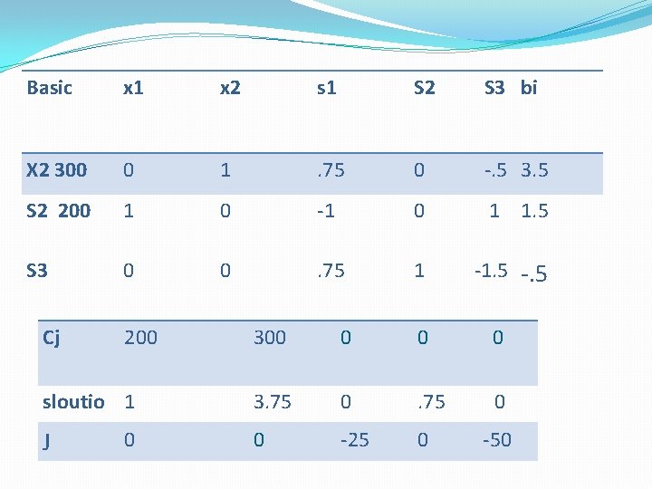
Basic x 1 x 2 s 1 S 2 S 3 bi X 2 300 0 1 . 75 0 -. 5 3. 5 S 2 200 1 0 -1 0 1 1. 5 S 3 0 0 . 75 1 -1. 5 -. 5 Cj 200 sloutio 1 J 0 300 0 3. 75 0 0 -25 0 -50

TAHNKS