Instrumental Analysis Statistics II IV Normal Error Law

Instrumental Analysis Statistics II

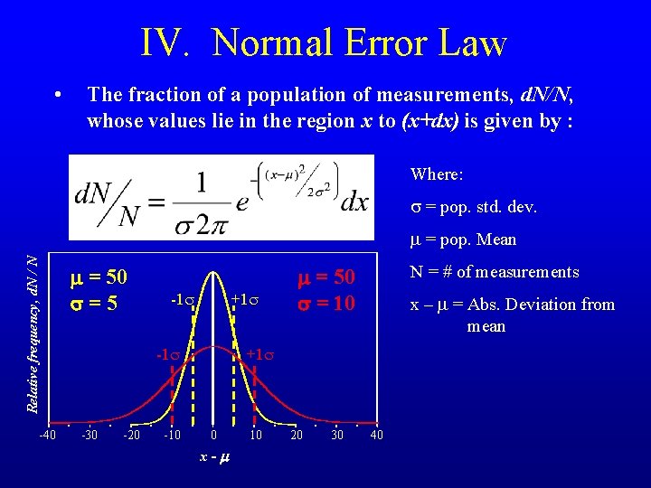
IV. Normal Error Law • The fraction of a population of measurements, d. N/N, whose values lie in the region x to (x+dx) is given by : Where: s = pop. std. dev. Relative frequency, d. N / N m = pop. Mean -40 m = 50 s=5 -1 s +1 s -30 -20 -10 N = # of measurements m = 50 s = 10 x – m = Abs. Deviation from mean +1 s 0 x-m 10 20 30 40

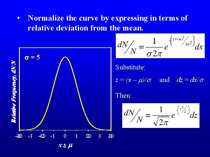
Relative Frequency, d. N/N • Normalize the curve by expressing in terms of relative deviation from the mean. s=5 -20 -4 -3 -10 -2 -1 Substitute: z = (x – m)/s Then: 0 x z- m 1 10 2 3 20 4 and dz = dx/s

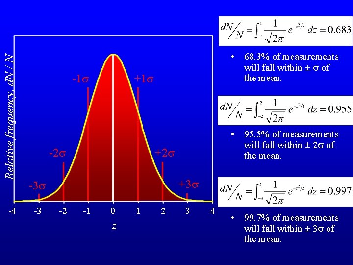
Relative frequency, d. N / N -4 -1 s • 68. 3% of measurements will fall within ± s of the mean. +1 s -2 s +3 s -3 • 95. 5% of measurements will fall within ± 2 s of the mean. -2 -1 0 z 1 2 3 4 • 99. 7% of measurements will fall within ± 3 s of the mean.

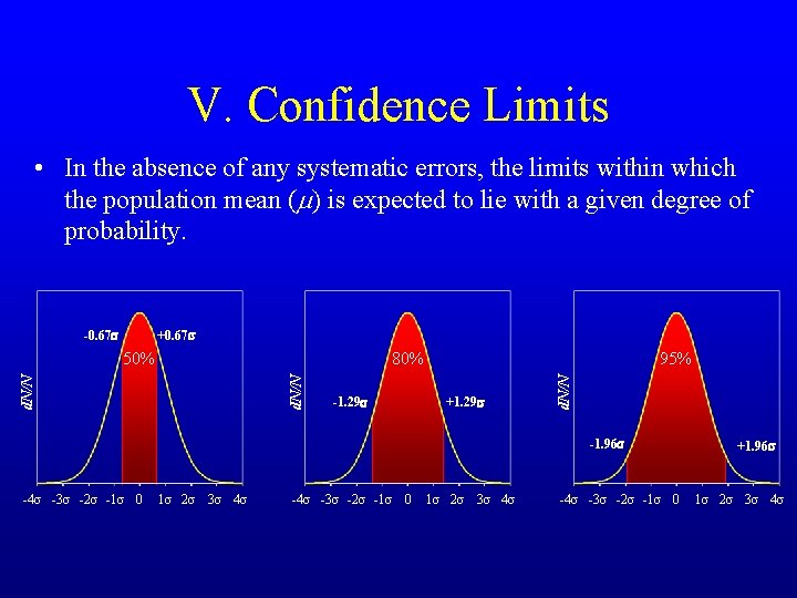
V. Confidence Limits • In the absence of any systematic errors, the limits within which the population mean (m) is expected to lie with a given degree of probability. +0. 67 s 95% 80% d. N/N 50% -1. 29 s +1. 29 s d. N/N -0. 67 s -1. 96 s -4 s -3 s -2 s -1 s 0 1 s 2 s 3 s 4 s -4 s -3 s -2 s -1 s 0 +1. 96 s 1 s 2 s 3 s 4 s

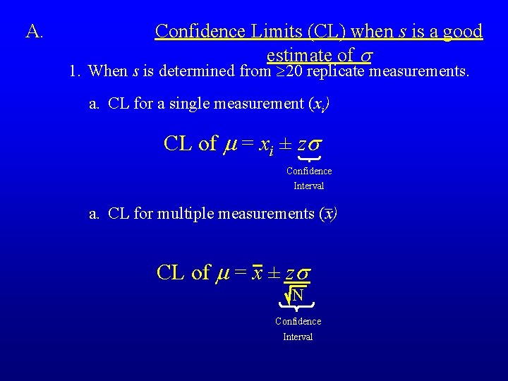
A. Confidence Limits (CL) when s is a good estimate of s 1. When s is determined from ³ 20 replicate measurements. a. CL for a single measurement (xi) CL of m = xi ± zs Confidence Interval a. CL for multiple measurements (x) CL of m = x ± zs N Confidence Interval

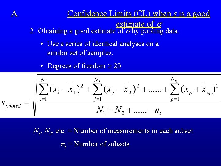
A. Confidence Limits (CL) when s is a good estimate of s 2. Obtaining a good estimate of s by pooling data. • Use a series of identical analyses on a similar set of samples. • Degrees of freedom ³ 20 N 1, N 2, etc. = Number of measurements in each subset nt = Number of subsets

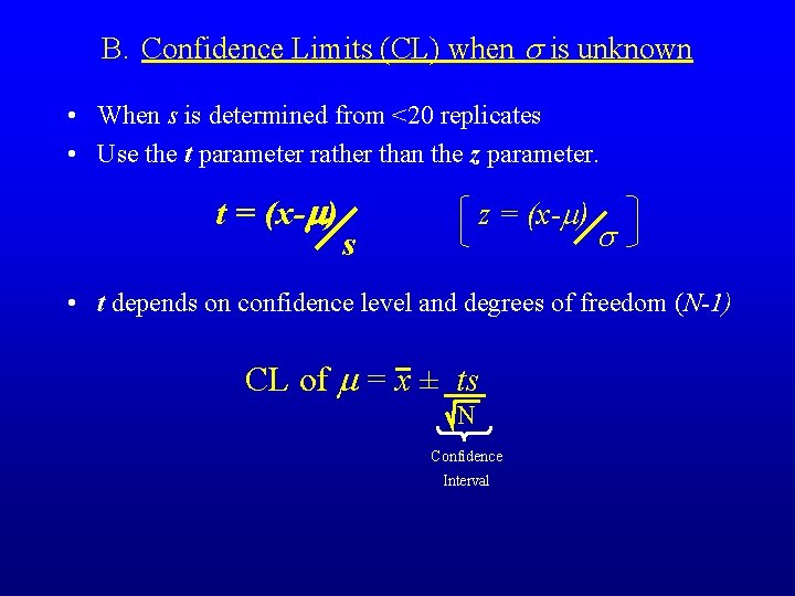
B. Confidence Limits (CL) when s is unknown • When s is determined from <20 replicates • Use the t parameter rather than the z parameter. t = (x-m) z = (x-m) s s • t depends on confidence level and degrees of freedom (N-1) CL of m = x ± ts N Confidence Interval

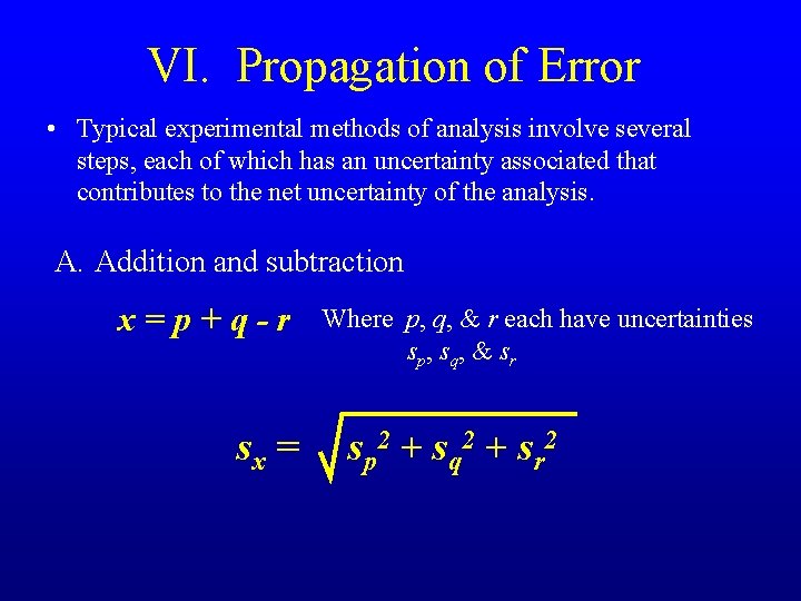
VI. Propagation of Error • Typical experimental methods of analysis involve several steps, each of which has an uncertainty associated that contributes to the net uncertainty of the analysis. A. Addition and subtraction x=p+q-r sx = Where p, q, & r each have uncertainties sp, sq, & sr sp 2 + sq 2 + sr 2

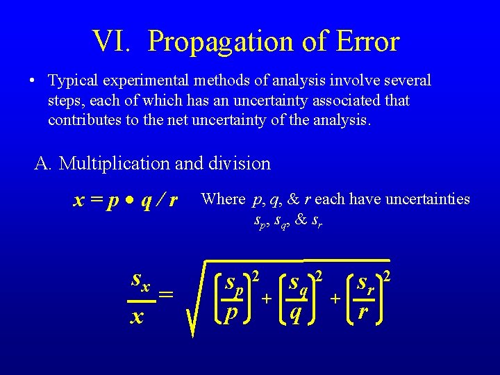
VI. Propagation of Error • Typical experimental methods of analysis involve several steps, each of which has an uncertainty associated that contributes to the net uncertainty of the analysis. A. Multiplication and division x=p·q/r sx x = Where p, q, & r each have uncertainties sp, sq, & sr sp p 2 + sq q 2 + sr r 2