INSTRUCTOR 2017 John R Fanchi All rights reserved

INSTRUCTOR © 2017, John R. Fanchi All rights reserved. No part of this manual may be reproduced in any form without the express written permission of the author.

To the Instructor The set of files here are designed to help you prepare lectures for your own course using the text Introduction to Petroleum Engineering, J. R. Fanchi and R. L. Christiansen (Wiley, 2017) File format is kept simple so that you can customize the files with relative ease using your own style. You will need to supplement the files to complete the presentation topics.

PERMEABILITY © 2017, John R. Fanchi All rights reserved. No part of this manual may be reproduced in any form without the express written permission of the author.

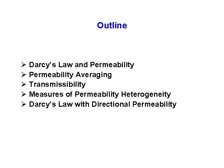
Outline Ø Darcy’s Law and Permeability Ø Permeability Averaging Ø Transmissibility Ø Measures of Permeability Heterogeneity Ø Darcy’s Law with Directional Permeability

DARCY’S LAW AND PERMEABILITY

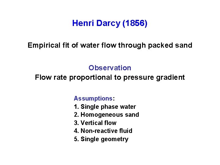
Henri Darcy (1856) Empirical fit of water flow through packed sand Observation Flow rate proportional to pressure gradient Assumptions: 1. Single phase water 2. Homogeneous sand 3. Vertical flow 4. Non-reactive fluid 5. Single geometry

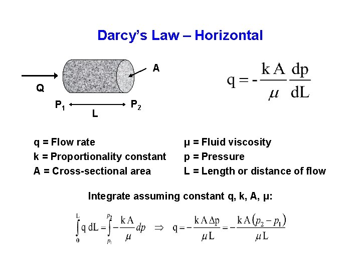
Darcy’s Law – Horizontal A Q P 1 L P 2 q = Flow rate k = Proportionality constant A = Cross-sectional area μ = Fluid viscosity p = Pressure L = Length or distance of flow Integrate assuming constant q, k, A, μ:

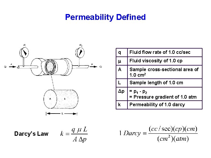
Permeability Defined Darcy’s Law q Fluid flow rate of 1. 0 cc/sec Fluid viscosity of 1. 0 cp A Sample cross-sectional area of 1. 0 cm 2 L Sample length of 1. 0 cm Δp = p 1 - p 2 = Pressure gradient of 1. 0 atm k Permeability of 1. 0 darcy

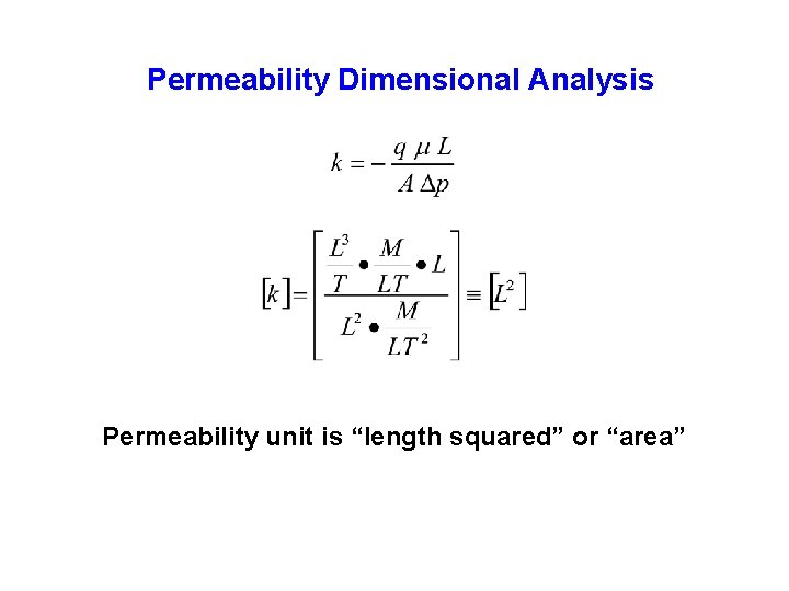
Permeability Dimensional Analysis Permeability unit is “length squared” or “area”

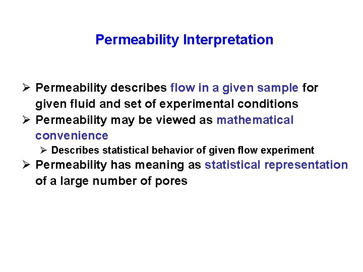
Permeability Interpretation Ø Permeability describes flow in a given sample for given fluid and set of experimental conditions Ø Permeability may be viewed as mathematical convenience Ø Describes statistical behavior of given flow experiment Ø Permeability has meaning as statistical representation of a large number of pores

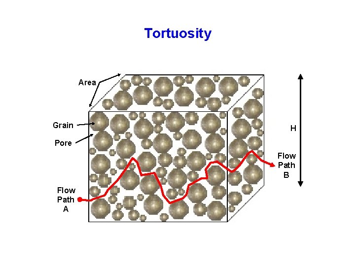
Tortuosity Area Grain H Pore Flow Path B Flow Path A

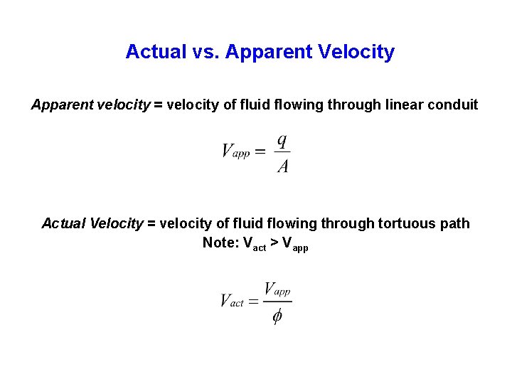
Actual vs. Apparent Velocity Apparent velocity = velocity of fluid flowing through linear conduit Actual Velocity = velocity of fluid flowing through tortuous path Note: Vact > Vapp

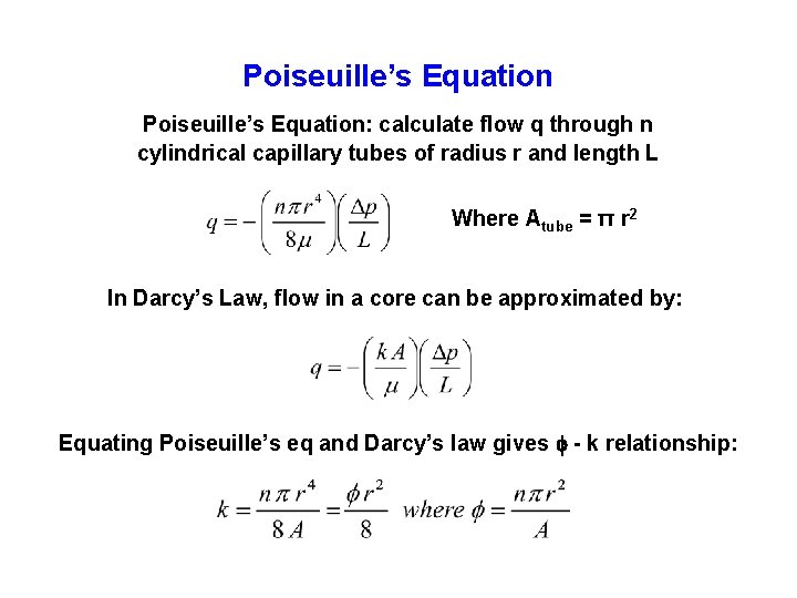
Poiseuille’s Equation: calculate flow q through n cylindrical capillary tubes of radius r and length L Where Atube = π r 2 In Darcy’s Law, flow in a core can be approximated by: Equating Poiseuille’s eq and Darcy’s law gives - k relationship:

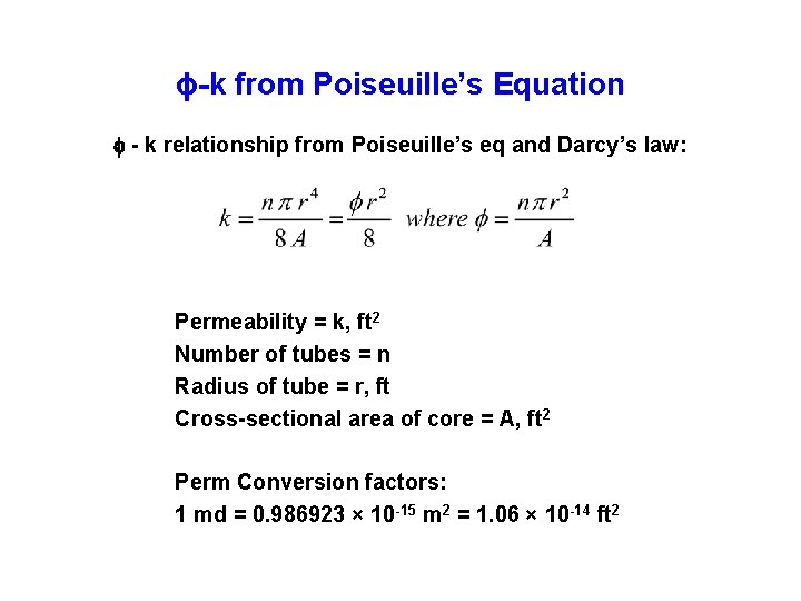
ϕ-k from Poiseuille’s Equation - k relationship from Poiseuille’s eq and Darcy’s law: Permeability = k, ft 2 Number of tubes = n Radius of tube = r, ft Cross-sectional area of core = A, ft 2 Perm Conversion factors: 1 md = 0. 986923 × 10 -15 m 2 = 1. 06 × 10 -14 ft 2

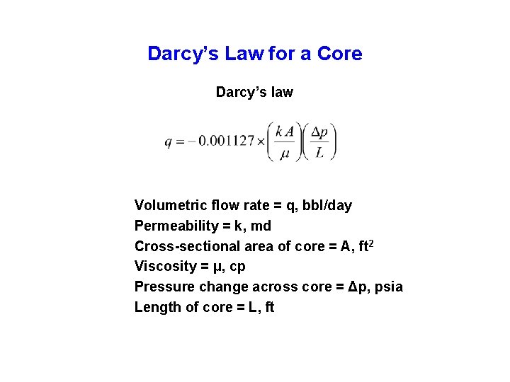
Darcy’s Law for a Core Darcy’s law Volumetric flow rate = q, bbl/day Permeability = k, md Cross-sectional area of core = A, ft 2 Viscosity = μ, cp Pressure change across core = Δp, psia Length of core = L, ft

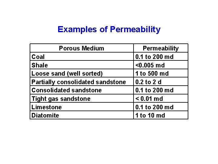
Examples of Permeability Porous Medium Coal Shale Loose sand (well sorted) Partially consolidated sandstone Consolidated sandstone Tight gas sandstone Limestone Diatomite Permeability 0. 1 to 200 md <0. 005 md 1 to 500 md 0. 2 to 2 d 0. 1 to 200 md < 0. 01 md 0. 1 to 200 md 1 to 10 md

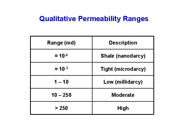
Qualitative Permeability Ranges Range (md) Description ≈ 10 -6 Shale (nanodarcy) ≈ 10 -3 Tight (microdarcy) 1 – 10 Low (millidarcy) 10 – 250 Moderate > 250 High

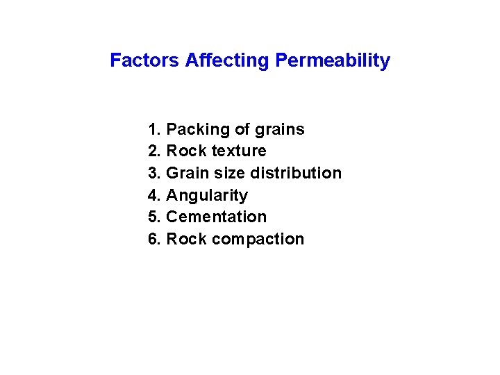
Factors Affecting Permeability 1. Packing of grains 2. Rock texture 3. Grain size distribution 4. Angularity 5. Cementation 6. Rock compaction

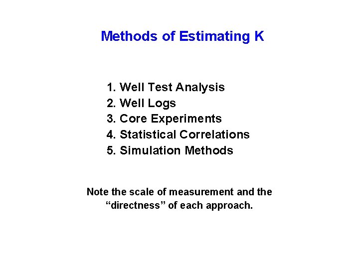
Methods of Estimating K 1. Well Test Analysis 2. Well Logs 3. Core Experiments 4. Statistical Correlations 5. Simulation Methods Note the scale of measurement and the “directness” of each approach.

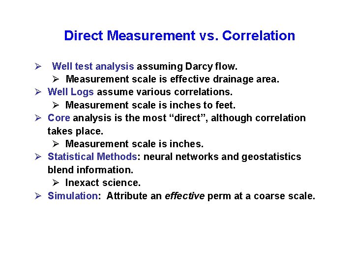
Direct Measurement vs. Correlation Ø Well test analysis assuming Darcy flow. Ø Measurement scale is effective drainage area. Ø Well Logs assume various correlations. Ø Measurement scale is inches to feet. Ø Core analysis is the most “direct”, although correlation takes place. Ø Measurement scale is inches. Ø Statistical Methods: neural networks and geostatistics blend information. Ø Inexact science. Ø Simulation: Attribute an effective perm at a coarse scale.

PERMEABILITY AVERAGING

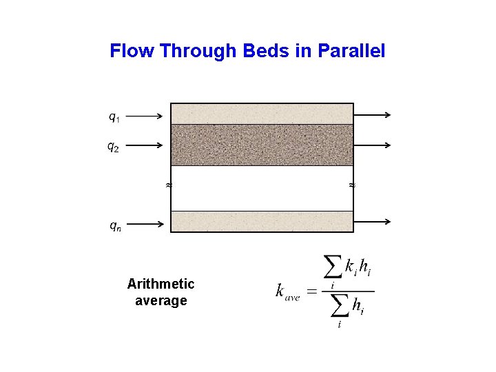
Flow Through Beds in Parallel Arithmetic average

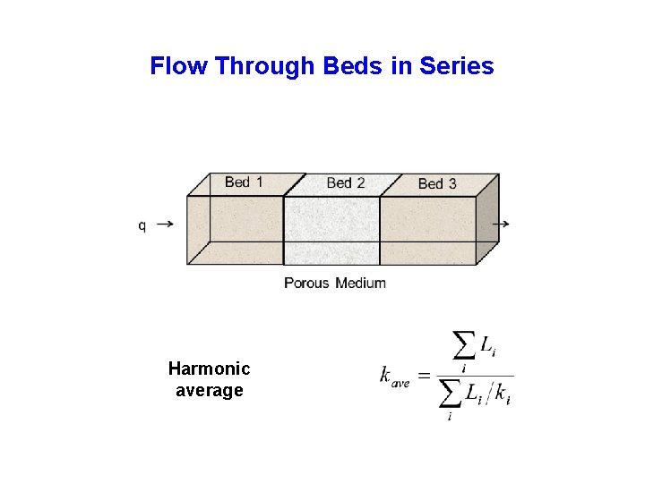
Flow Through Beds in Series Harmonic average

TRANSMISSIBILITY

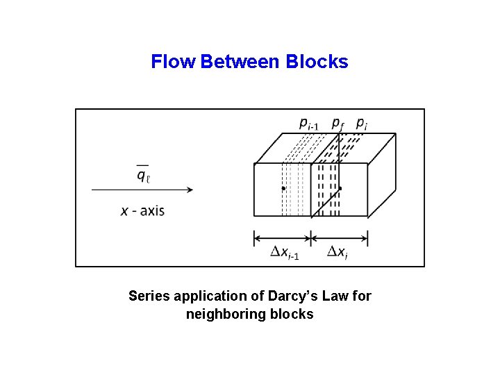
Flow Between Blocks Series application of Darcy’s Law for neighboring blocks

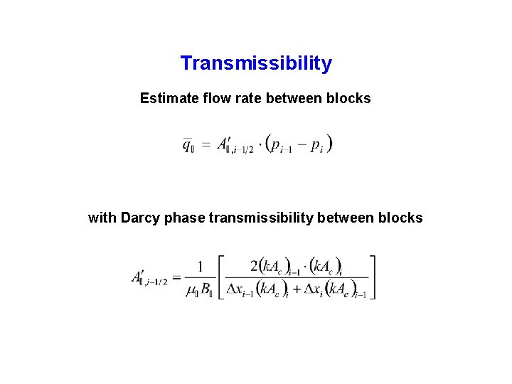
Transmissibility Estimate flow rate between blocks with Darcy phase transmissibility between blocks

MEASURES OF PERMEABILITY HETEROGENEITY

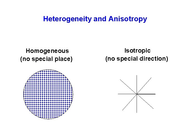
Heterogeneity and Anisotropy Homogeneous (no special place) Isotropic (no special direction)

HETEROGENEITY MEASURES Heterogeneity: Spatial variability of permeability DYKSTRA-PARSONS COEFFICIENT (SPE 20156, Lake and Jensen, 1989) LORENZ COEFFICIENT (SPE 20156, Lake and Jensen, 1989)

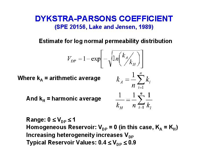
DYKSTRA-PARSONS COEFFICIENT (SPE 20156, Lake and Jensen, 1989) Estimate for log normal permeability distribution Where k. A = arithmetic average And k. H = harmonic average Range: 0 VDP 1 Homogeneous Reservoir: VDP = 0 (in this case, KA = KH) Increasing heterogeneity increases VDP Typical Reservoir Values: 0. 4 VDP 0. 9

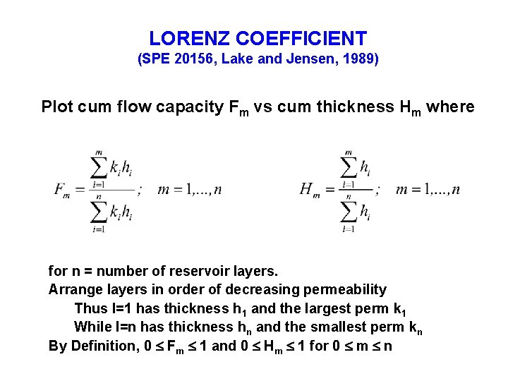
LORENZ COEFFICIENT (SPE 20156, Lake and Jensen, 1989) Plot cum flow capacity Fm vs cum thickness Hm where for n = number of reservoir layers. Arrange layers in order of decreasing permeability Thus I=1 has thickness h 1 and the largest perm k 1 While I=n has thickness hn and the smallest perm kn By Definition, 0 Fm 1 and 0 Hm 1 for 0 m n

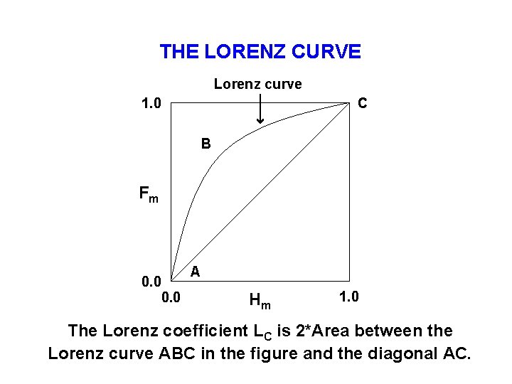
THE LORENZ CURVE Lorenz curve 1. 0 C B Fm 0. 0 A Hm 1. 0 The Lorenz coefficient LC is 2*Area between the Lorenz curve ABC in the figure and the diagonal AC.

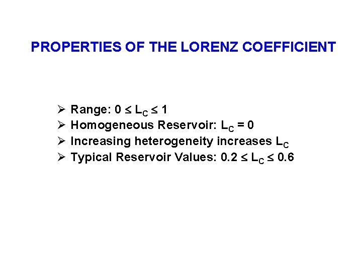
PROPERTIES OF THE LORENZ COEFFICIENT Ø Ø Range: 0 LC 1 Homogeneous Reservoir: LC = 0 Increasing heterogeneity increases LC Typical Reservoir Values: 0. 2 LC 0. 6

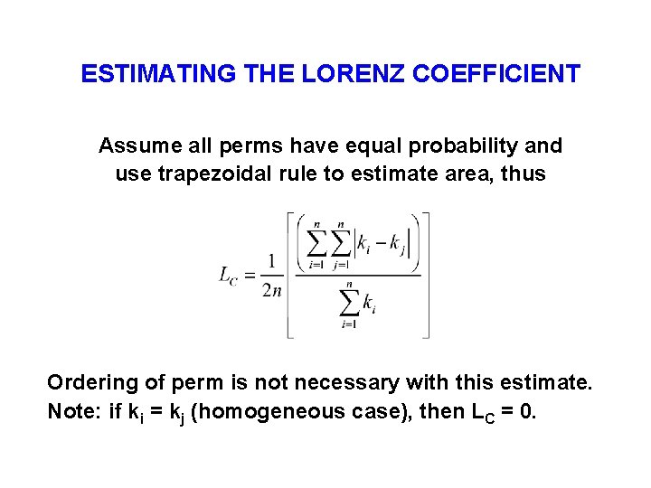
ESTIMATING THE LORENZ COEFFICIENT Assume all perms have equal probability and use trapezoidal rule to estimate area, thus Ordering of perm is not necessary with this estimate. Note: if ki = kj (homogeneous case), then LC = 0.

DARCY’S LAW WITH DIRECTIONAL PERMEABILITY

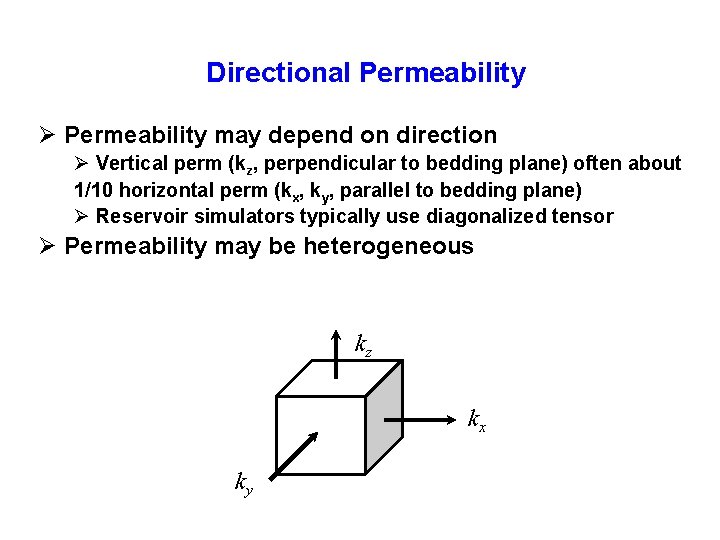
Directional Permeability Ø Permeability may depend on direction Ø Vertical perm (kz, perpendicular to bedding plane) often about 1/10 horizontal perm (kx, ky, parallel to bedding plane) Ø Reservoir simulators typically use diagonalized tensor Ø Permeability may be heterogeneous kz kx ky

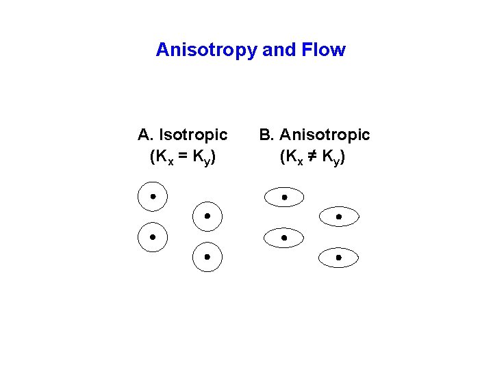
Anisotropy and Flow A. Isotropic (Kx = Ky) B. Anisotropic (Kx ≠ Ky)

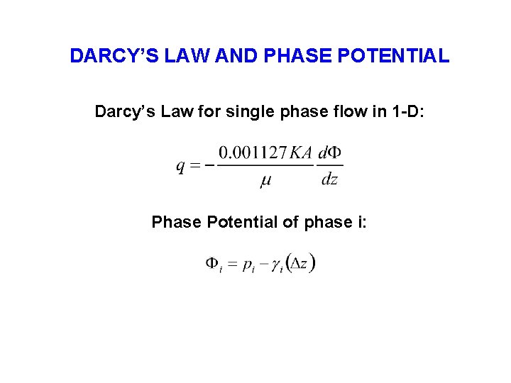
DARCY’S LAW AND PHASE POTENTIAL Darcy’s Law for single phase flow in 1 -D: Phase Potential of phase i:

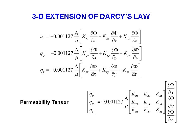
3 -D EXTENSION OF DARCY’S LAW Permeability Tensor

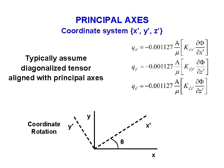
PRINCIPAL AXES Coordinate system {x’, y’, z’} Typically assume diagonalized tensor aligned with principal axes y Coordinate Rotation x' y' θ x

QUESTIONS?

SUPPLEMENT