Insertion Sorting Analysis 1 Insertion Sort sorted part

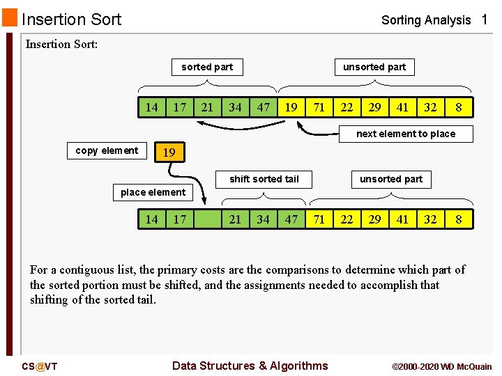
Insertion Sorting Analysis 1 Insertion Sort: sorted part 14 17 21 34 unsorted part 47 19 71 22 29 41 32 8 next element to place copy element 19 shift sorted tail unsorted part place element 14 17 21 34 47 71 22 29 41 32 8 For a contiguous list, the primary costs are the comparisons to determine which part of the sorted portion must be shifted, and the assignments needed to accomplish that shifting of the sorted tail. CS@VT Data Structures & Algorithms © 2000 -2020 WD Mc. Quain

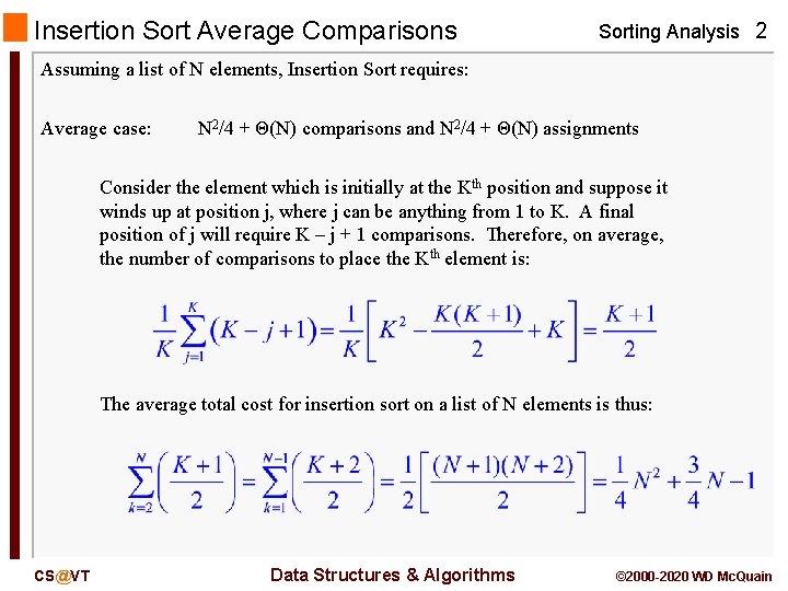
Insertion Sort Average Comparisons Sorting Analysis 2 Assuming a list of N elements, Insertion Sort requires: Average case: N 2/4 + Θ(N) comparisons and N 2/4 + Θ(N) assignments Consider the element which is initially at the Kth position and suppose it winds up at position j, where j can be anything from 1 to K. A final position of j will require K – j + 1 comparisons. Therefore, on average, the number of comparisons to place the Kth element is: The average total cost for insertion sort on a list of N elements is thus: CS@VT Data Structures & Algorithms © 2000 -2020 WD Mc. Quain

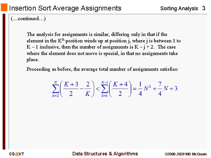
Insertion Sort Average Assignments Sorting Analysis 3 (…continued…) The analysis for assignments is similar, differing only in that if the element in the Kth position winds up at position j, where j is between 1 to K – 1 inclusive, then the number of assignments is K – j + 2. The case where the element does not move is special, in that no assignments take place. Proceeding as before, the average total number of assignments satisfies: CS@VT Data Structures & Algorithms © 2000 -2020 WD Mc. Quain

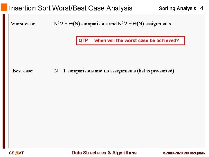
Insertion Sort Worst/Best Case Analysis Worst case: Sorting Analysis 4 N 2/2 + Θ(N) comparisons and N 2/2 + Θ(N) assignments QTP: when will the worst case be achieved? Best case: CS@VT N – 1 comparisons and no assignments (list is pre-sorted) Data Structures & Algorithms © 2000 -2020 WD Mc. Quain

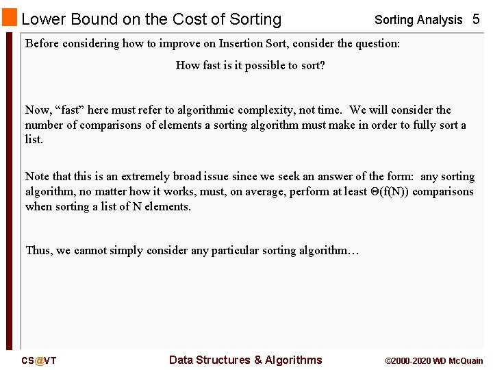
Lower Bound on the Cost of Sorting Analysis 5 Before considering how to improve on Insertion Sort, consider the question: How fast is it possible to sort? Now, “fast” here must refer to algorithmic complexity, not time. We will consider the number of comparisons of elements a sorting algorithm must make in order to fully sort a list. Note that this is an extremely broad issue since we seek an answer of the form: any sorting algorithm, no matter how it works, must, on average, perform at least Θ(f(N)) comparisons when sorting a list of N elements. Thus, we cannot simply consider any particular sorting algorithm… CS@VT Data Structures & Algorithms © 2000 -2020 WD Mc. Quain

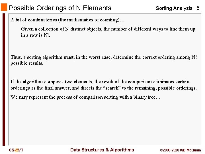
Possible Orderings of N Elements Sorting Analysis 6 A bit of combinatorics (the mathematics of counting)… Given a collection of N distinct objects, the number of different ways to line them up in a row is N!. Thus, a sorting algorithm must, in the worst case, determine the correct ordering among N! possible results. If the algorithm compares two elements, the result of the comparison eliminates certain orderings as the final answer, and directs the “search” to the remaining, possible orderings. We may represent the process of comparison sorting with a binary tree… CS@VT Data Structures & Algorithms © 2000 -2020 WD Mc. Quain

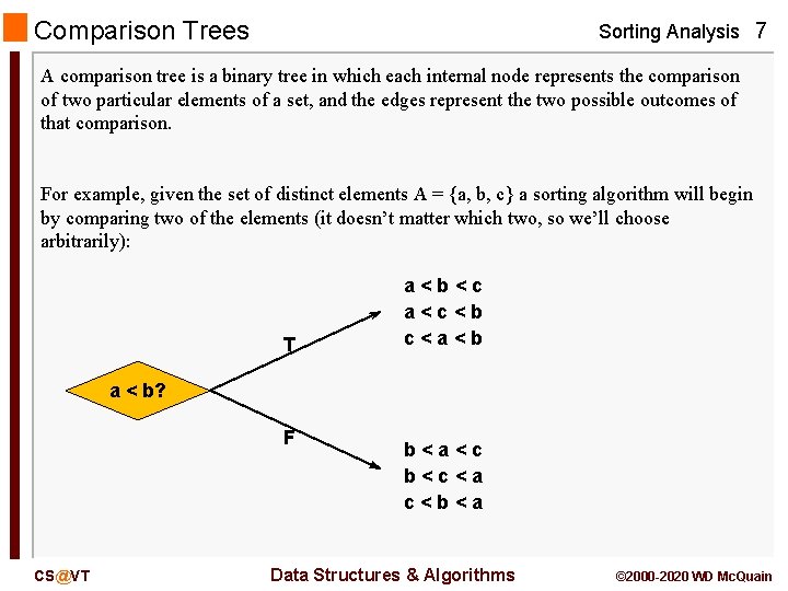
Comparison Trees Sorting Analysis 7 A comparison tree is a binary tree in which each internal node represents the comparison of two particular elements of a set, and the edges represent the two possible outcomes of that comparison. For example, given the set of distinct elements A = {a, b, c} a sorting algorithm will begin by comparing two of the elements (it doesn’t matter which two, so we’ll choose arbitrarily): T a<b<c a<c<b c<a<b a < b? F CS@VT b<a<c b<c<a c<b<a Data Structures & Algorithms © 2000 -2020 WD Mc. Quain

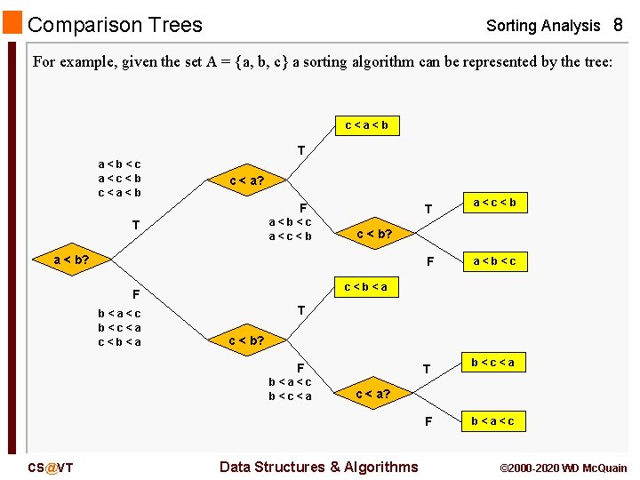
Comparison Trees Sorting Analysis 8 For example, given the set A = {a, b, c} a sorting algorithm can be represented by the tree: c<a<b T a<b<c a<c<b c<a<b c < a? F a<b<c a<c<b T T c < b? a < b? F T c < b? F b<a<c b<c<a T b<c<a c < a? F CS@VT a<b<c c<b<a F b<a<c b<c<a c<b<a a<c<b Data Structures & Algorithms b<a<c © 2000 -2020 WD Mc. Quain

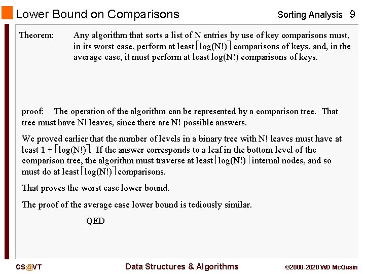
Lower Bound on Comparisons Theorem: Sorting Analysis 9 Any algorithm that sorts a list of N entries by use of key comparisons must, in its worst case, perform at least log(N!) comparisons of keys, and, in the average case, it must perform at least log(N!) comparisons of keys. proof: The operation of the algorithm can be represented by a comparison tree. That tree must have N! leaves, since there are N! possible answers. We proved earlier that the number of levels in a binary tree with N! leaves must have at least 1 + log(N!). If the answer corresponds to a leaf in the bottom level of the comparison tree, the algorithm must traverse at least log(N!) internal nodes, and so must do at least log(N!) comparisons. That proves the worst case lower bound. The proof of the average case lower bound is tediously similar. QED CS@VT Data Structures & Algorithms © 2000 -2020 WD Mc. Quain

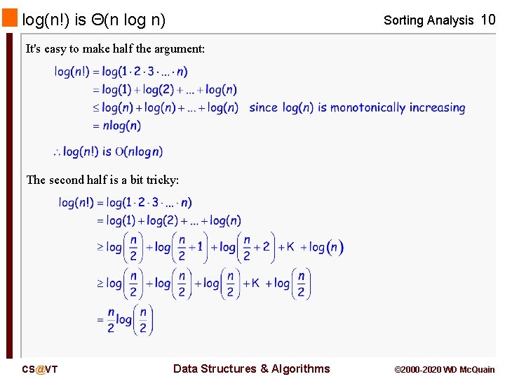
log(n!) is Θ(n log n) Sorting Analysis 10 It's easy to make half the argument: The second half is a bit tricky: CS@VT Data Structures & Algorithms © 2000 -2020 WD Mc. Quain

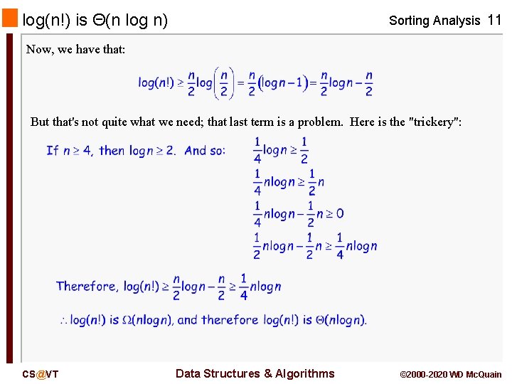
log(n!) is Θ(n log n) Sorting Analysis 11 Now, we have that: But that's not quite what we need; that last term is a problem. Here is the "trickery": CS@VT Data Structures & Algorithms © 2000 -2020 WD Mc. Quain

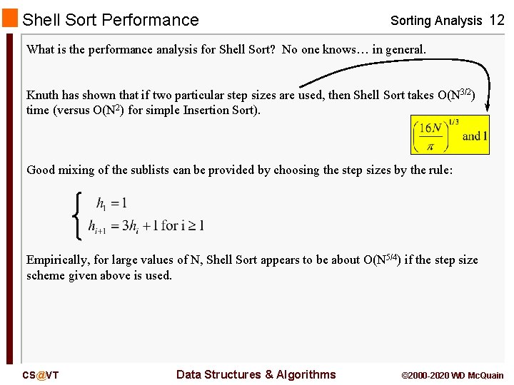
Shell Sort Performance Sorting Analysis 12 What is the performance analysis for Shell Sort? No one knows… in general. Knuth has shown that if two particular step sizes are used, then Shell Sort takes O(N 3/2) time (versus O(N 2) for simple Insertion Sort). Good mixing of the sublists can be provided by choosing the step sizes by the rule: Empirically, for large values of N, Shell Sort appears to be about O(N 5/4) if the step size scheme given above is used. CS@VT Data Structures & Algorithms © 2000 -2020 WD Mc. Quain

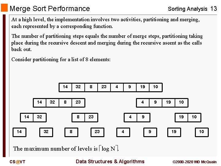
Merge Sort Performance Sorting Analysis 13 At a high level, the implementation involves two activities, partitioning and merging, each represented by a corresponding function. The number of partitioning steps equals the number of merge steps, partitioning taking place during the recursive descent and merging during the recursive ascent as the calls back out. Consider partitioning for a list of 8 elements: 14 14 14 32 8 23 32 8 8 23 4 9 23 4 23 19 10 4 9 19 10 9 4 19 9 19 10 10 The maximum number of levels is log N. CS@VT Data Structures & Algorithms © 2000 -2020 WD Mc. Quain

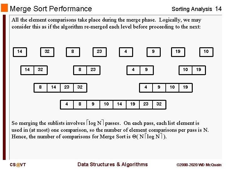
Merge Sort Performance Sorting Analysis 14 All the element comparisons take place during the merge phase. Logically, we may consider this as if the algorithm re-merged each level before proceeding to the next: 14 32 14 8 32 8 23 8 14 23 32 4 8 4 23 9 9 4 10 14 19 19 9 10 10 4 9 23 32 10 19 19 So merging the sublists involves log N passes. On each pass, each list element is used in (at most) one comparison, so the number of element comparisons per pass is N. Hence, the number of comparisons for Merge Sort is Θ( N log N ). CS@VT Data Structures & Algorithms © 2000 -2020 WD Mc. Quain

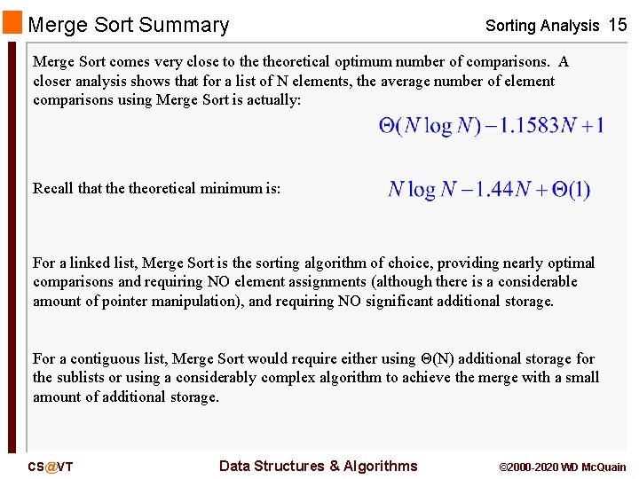
Merge Sort Summary Sorting Analysis 15 Merge Sort comes very close to theoretical optimum number of comparisons. A closer analysis shows that for a list of N elements, the average number of element comparisons using Merge Sort is actually: Recall that theoretical minimum is: For a linked list, Merge Sort is the sorting algorithm of choice, providing nearly optimal comparisons and requiring NO element assignments (although there is a considerable amount of pointer manipulation), and requiring NO significant additional storage. For a contiguous list, Merge Sort would require either using Θ(N) additional storage for the sublists or using a considerably complex algorithm to achieve the merge with a small amount of additional storage. CS@VT Data Structures & Algorithms © 2000 -2020 WD Mc. Quain

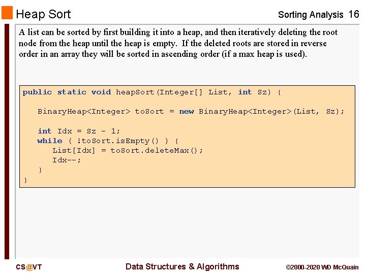
Heap Sorting Analysis 16 A list can be sorted by first building it into a heap, and then iteratively deleting the root node from the heap until the heap is empty. If the deleted roots are stored in reverse order in an array they will be sorted in ascending order (if a max heap is used). public static void heap. Sort(Integer[] List, int Sz) { Binary. Heap<Integer> to. Sort = new Binary. Heap<Integer>(List, Sz); int Idx = Sz - 1; while ( !to. Sort. is. Empty() ) { List[Idx] = to. Sort. delete. Max(); Idx--; } } CS@VT Data Structures & Algorithms © 2000 -2020 WD Mc. Quain

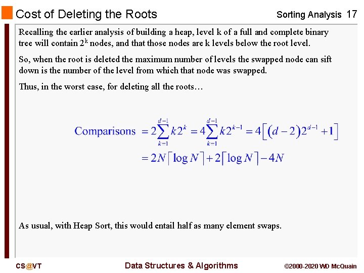
Cost of Deleting the Roots Sorting Analysis 17 Recalling the earlier analysis of building a heap, level k of a full and complete binary tree will contain 2 k nodes, and that those nodes are k levels below the root level. So, when the root is deleted the maximum number of levels the swapped node can sift down is the number of the level from which that node was swapped. Thus, in the worst case, for deleting all the roots… As usual, with Heap Sort, this would entail half as many element swaps. CS@VT Data Structures & Algorithms © 2000 -2020 WD Mc. Quain

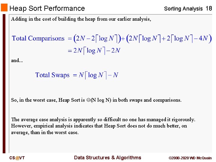
Heap Sort Performance Sorting Analysis 18 Adding in the cost of building the heap from our earlier analysis, and. . . So, in the worst case, Heap Sort is (N log N) in both swaps and comparisons. The average case analysis is apparently so difficult no one has managed it rigorously. However, empirical analysis indicates that Heap Sort does not do much better, on average, than in the worst case. CS@VT Data Structures & Algorithms © 2000 -2020 WD Mc. Quain

Quick. Sort Performance Sorting Analysis 19 As with Merge Sort, we can view Quick. Sort as consisting of a sequence of steps, each involving pivot selection and then partitioning of each nontrivial sublist. What is the total partitioning cost at each step? As implemented here, each partitioning step isolates a copy of the pivot value and that value is not subsequently moved, so the number of elements that are subject to partitioning decreases at each step. However, it is relatively clear that the total cost of partitioning at any step is no worse than Θ(N). But, how many steps must be performed? Ah, there’s the rub… that depends upon how well the pivot values work. CS@VT Data Structures & Algorithms © 2000 -2020 WD Mc. Quain

Quick. Sort Performance Analysis Sorting Analysis 20 For simplicity in analysis, we will make the following assumptions: - the key values to be partitioned are 1…N - C(N) is the number of comparisons made by Quick. Sort when applied to a list of length N - S(N) is the number of swaps made by Quick. Sort when applied to a list of length N If partitioning produces one sublist of length r and one of N – r – 1, then: C(N) = N – 1 + C(r) + C(N – r – 1) since the initial partition will require N – 1 element comparisons. The formula derived here is known as a recurrence relation. For a given value of r, it is possible to solve for C(N)… CS@VT Data Structures & Algorithms © 2000 -2020 WD Mc. Quain

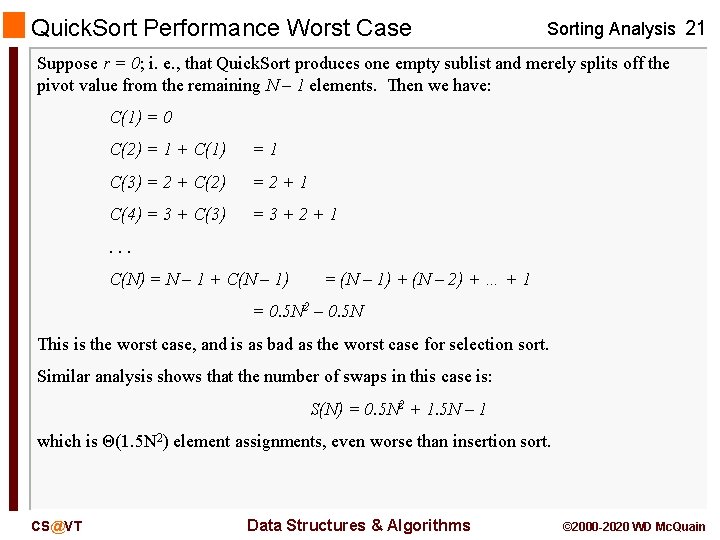
Quick. Sort Performance Worst Case Sorting Analysis 21 Suppose r = 0; i. e. , that Quick. Sort produces one empty sublist and merely splits off the pivot value from the remaining N – 1 elements. Then we have: C(1) = 0 C(2) = 1 + C(1) =1 C(3) = 2 + C(2) =2+1 C(4) = 3 + C(3) =3+2+1 . . . C(N) = N – 1 + C(N – 1) = (N – 1) + (N – 2) + … + 1 = 0. 5 N 2 – 0. 5 N This is the worst case, and is as bad as the worst case for selection sort. Similar analysis shows that the number of swaps in this case is: S(N) = 0. 5 N 2 + 1. 5 N – 1 which is Θ(1. 5 N 2) element assignments, even worse than insertion sort. CS@VT Data Structures & Algorithms © 2000 -2020 WD Mc. Quain

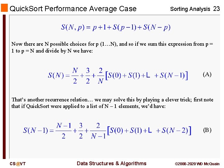
Quick. Sort Performance Average Case Sorting Analysis 22 For the average case, we will consider all possible results of the partitioning phase and compute the average of those. We assume that all possible orderings of the list elements are equally likely to be the correct sorted order, and let p denote the pivot value chosen. Thus, after partitioning, recalling we assume the key values are 1…N, the values 1, … p – 1 are to the left of p, and the values p + 1, … N are to the right of p. Let S(N) be the average number of swaps made by Quick. Sort on a list of length N, and S(N, p) be the average number of swaps if the value p is chosen as the initial pivot. The partition implementation given here will perform p – 1 swaps within the loop, and two more outside the loop. Therefore… CS@VT Data Structures & Algorithms © 2000 -2020 WD Mc. Quain

Quick. Sort Performance Average Case Sorting Analysis 23 Now there are N possible choices for p (1…N), and so if we sum this expression from p = 1 to p = N and divide by N we have: (A) That’s another recurrence relation… we may solve this by playing a clever trick; first note that if Quick. Sort were applied to a list of N – 1 elements, we’d have: (B) CS@VT Data Structures & Algorithms © 2000 -2020 WD Mc. Quain

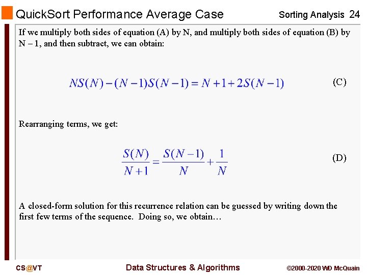
Quick. Sort Performance Average Case Sorting Analysis 24 If we multiply both sides of equation (A) by N, and multiply both sides of equation (B) by N – 1, and then subtract, we can obtain: (C) Rearranging terms, we get: (D) A closed-form solution for this recurrence relation can be guessed by writing down the first few terms of the sequence. Doing so, we obtain… CS@VT Data Structures & Algorithms © 2000 -2020 WD Mc. Quain

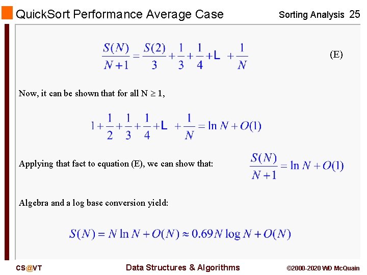
Quick. Sort Performance Average Case Sorting Analysis 25 (E) Now, it can be shown that for all N 1, Applying that fact to equation (E), we can show that: Algebra and a log base conversion yield: CS@VT Data Structures & Algorithms © 2000 -2020 WD Mc. Quain

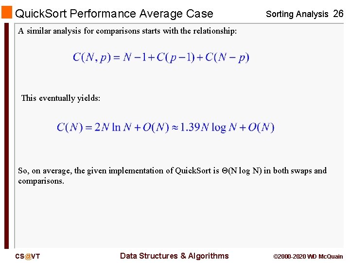
Quick. Sort Performance Average Case Sorting Analysis 26 A similar analysis for comparisons starts with the relationship: This eventually yields: So, on average, the given implementation of Quick. Sort is Θ(N log N) in both swaps and comparisons. CS@VT Data Structures & Algorithms © 2000 -2020 WD Mc. Quain

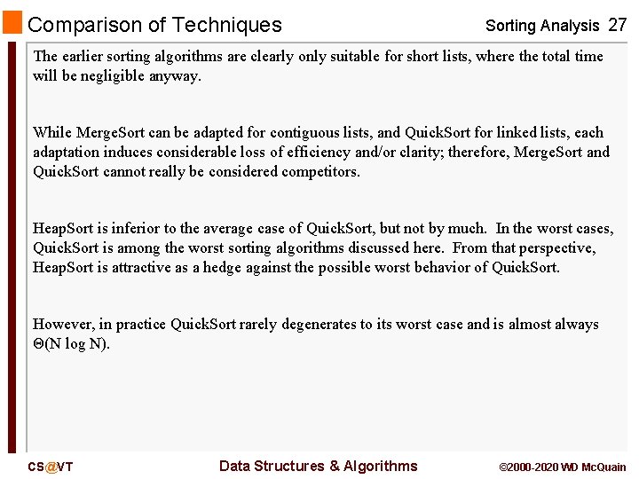
Comparison of Techniques Sorting Analysis 27 The earlier sorting algorithms are clearly only suitable for short lists, where the total time will be negligible anyway. While Merge. Sort can be adapted for contiguous lists, and Quick. Sort for linked lists, each adaptation induces considerable loss of efficiency and/or clarity; therefore, Merge. Sort and Quick. Sort cannot really be considered competitors. Heap. Sort is inferior to the average case of Quick. Sort, but not by much. In the worst cases, Quick. Sort is among the worst sorting algorithms discussed here. From that perspective, Heap. Sort is attractive as a hedge against the possible worst behavior of Quick. Sort. However, in practice Quick. Sort rarely degenerates to its worst case and is almost always Θ(N log N). CS@VT Data Structures & Algorithms © 2000 -2020 WD Mc. Quain

Beating the N log(N) Barrier Sorting Analysis 28 Theoretical analysis tells us that no sorting algorithm can require fewer comparisons than Θ(N log N), in its average case, right? Well, actually no… the derivation of that result assumes that the algorithm works by comparing key values. It is possible to devise sorting algorithms that do not compare the elements of the list to each other. In that case, the earlier result does not apply. However, such algorithms require special assumptions regarding the type and/or range of the key values to be sorted. CS@VT Data Structures & Algorithms © 2000 -2020 WD Mc. Quain

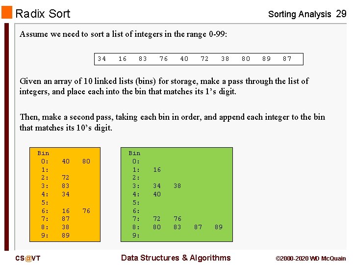
Radix Sorting Analysis 29 Assume we need to sort a list of integers in the range 0 -99: 34 16 83 76 40 72 38 80 89 87 Given an array of 10 linked lists (bins) for storage, make a pass through the list of integers, and place each into the bin that matches its 1’s digit. Then, make a second pass, taking each bin in order, and append each integer to the bin that matches its 10’s digit. Bin 0: 1: 2: 3: 4: 5: 6: 7: 8: 9: CS@VT 40 80 72 83 34 16 87 38 89 76 Bin 0: 1: 2: 3: 4: 5: 6: 7: 8: 9: 16 34 40 38 72 80 76 83 87 89 Data Structures & Algorithms © 2000 -2020 WD Mc. Quain

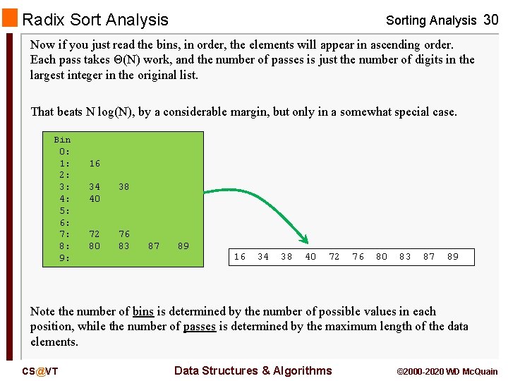
Radix Sort Analysis Sorting Analysis 30 Now if you just read the bins, in order, the elements will appear in ascending order. Each pass takes Θ(N) work, and the number of passes is just the number of digits in the largest integer in the original list. That beats N log(N), by a considerable margin, but only in a somewhat special case. Bin 0: 1: 2: 3: 4: 5: 6: 7: 8: 9: 16 34 40 38 72 80 76 83 87 89 16 34 38 40 72 76 80 83 87 89 Note the number of bins is determined by the number of possible values in each position, while the number of passes is determined by the maximum length of the data elements. CS@VT Data Structures & Algorithms © 2000 -2020 WD Mc. Quain