Insertion Sort The Sorting Problem Input A sequence

Insertion Sort

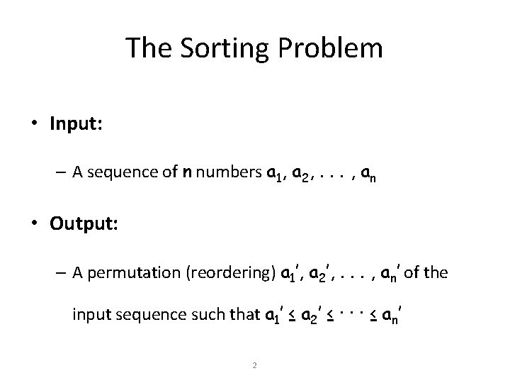
The Sorting Problem • Input: – A sequence of n numbers a 1, a 2, . . . , an • Output: – A permutation (reordering) a 1’, a 2’, . . . , an’ of the input sequence such that a 1’ ≤ a 2’ ≤ · · · ≤ an’ 2

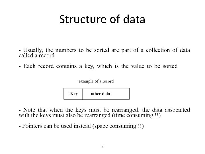
Structure of data 3

Why Study Sorting Algorithms? • There a variety of situations that we can encounter – Do we have randomly ordered keys? – Are all keys distinct? – How large is the set of keys to be ordered? – Need guaranteed performance? • Various algorithms are better suited to some of these situations 4

Some Definitions • Internal Sort – The data to be sorted is all stored in the computer’s main memory. • External Sort – Some of the data to be sorted might be stored in some external, slower, device. • In Place Sort – The amount of extra space required to sort the data is constant with the input size. 5

Stability • A STABLE sort preserves relative order of records with equal keys Sorted on first key: Sort file on second key: Records with key value 3 are not in order on first key!! 6

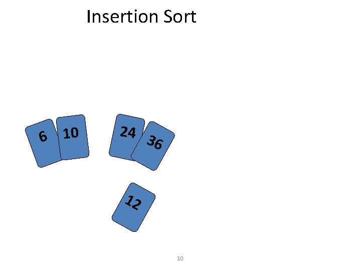
Insertion Sort • Idea: like sorting a hand of playing cards – Start with an empty left hand the cards facing down on the table. – Remove one card at a time from the table, and insert it into the correct position in the left hand • compare it with each of the cards already in the hand, from right to left – The cards held in the left hand are sorted • these cards were originally the top cards of the pile on the table 7

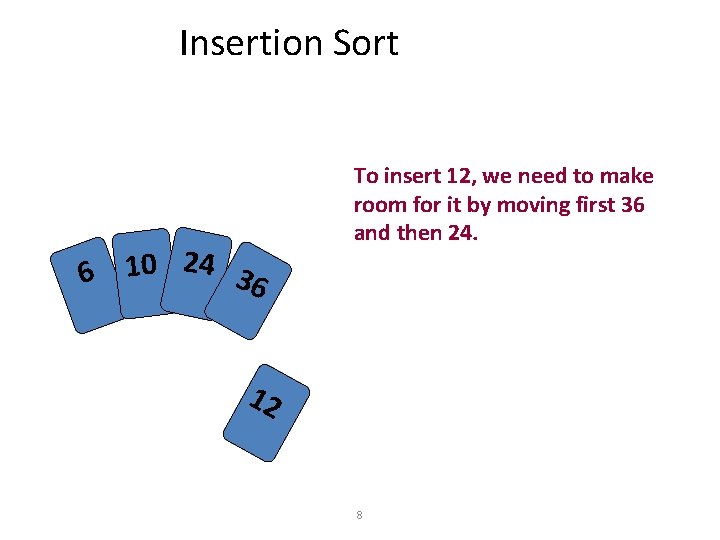
Insertion Sort 6 10 24 36 To insert 12, we need to make room for it by moving first 36 and then 24. 12 8

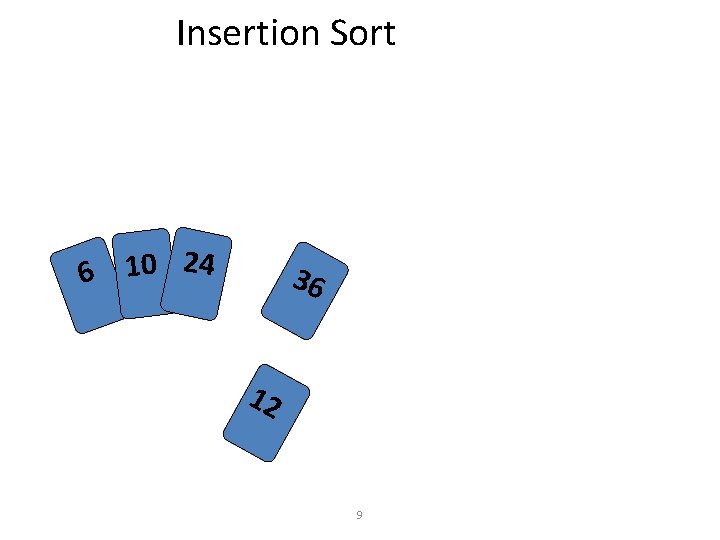
Insertion Sort 6 10 24 36 12 9

Insertion Sort 6 10 24 3 6 12 10

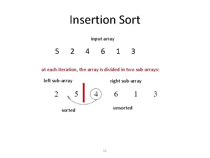
Insertion Sort input array 5 2 4 6 1 3 at each iteration, the array is divided in two sub-arrays: left sub-array right sub-array unsorted 11

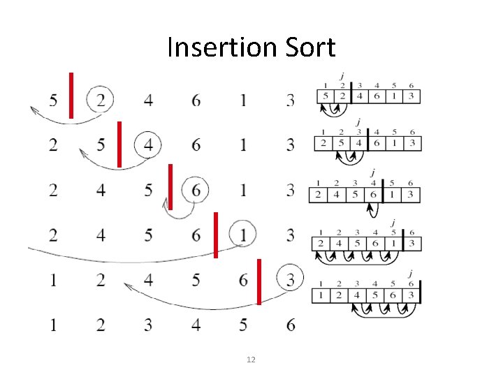
Insertion Sort 12

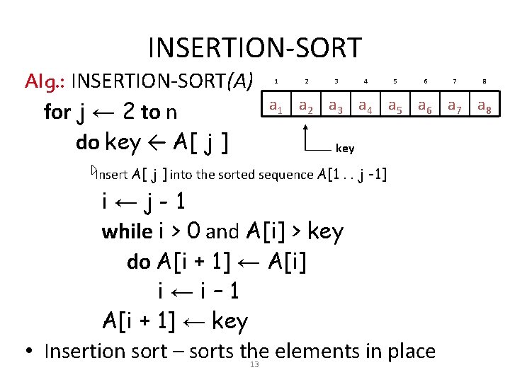
INSERTION-SORT Alg. : INSERTION-SORT(A) for j ← 2 to n do key ← A[ j ] 1 2 3 4 5 6 8 a 1 a 2 a 3 a 4 a 5 a 6 a 7 a 8 key Insert A[ j ] into the sorted sequence A[1. . j -1] i←j-1 while i > 0 and A[i] > key do A[i + 1] ← A[i] i←i– 1 A[i + 1] ← key • Insertion sort – sorts the elements in place 13 7

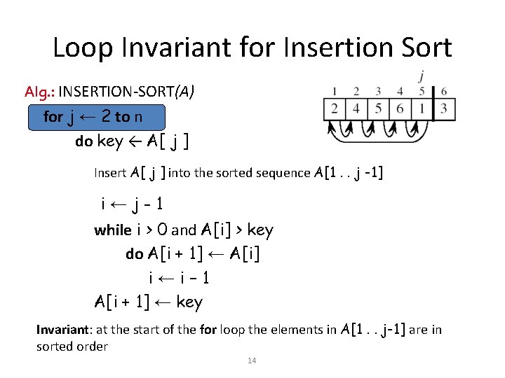
Loop Invariant for Insertion Sort Alg. : INSERTION-SORT(A) for j ← 2 to n do key ← A[ j ] Insert A[ j ] into the sorted sequence A[1. . j -1] i←j-1 while i > 0 and A[i] > key do A[i + 1] ← A[i] i←i– 1 A[i + 1] ← key Invariant: at the start of the for loop the elements in A[1. . j-1] are in sorted order 14

Proving Loop Invariants • Proving loop invariants works like induction • Initialization (base case): – It is true prior to the first iteration of the loop • Maintenance (inductive step): – If it is true before an iteration of the loop, it remains true before the next iteration • Termination: – When the loop terminates, the invariant gives us a useful property that helps show that the algorithm is correct – Stop the induction when the loop terminates 15

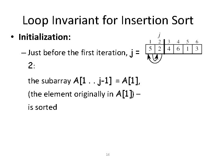
Loop Invariant for Insertion Sort • Initialization: – Just before the first iteration, j = 2: the subarray A[1. . j-1] = A[1], (the element originally in A[1]) – is sorted 16

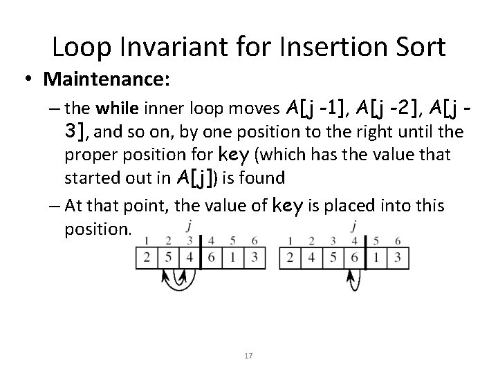
Loop Invariant for Insertion Sort • Maintenance: – the while inner loop moves A[j -1], A[j -2], A[j 3], and so on, by one position to the right until the proper position for key (which has the value that started out in A[j]) is found – At that point, the value of key is placed into this position. 17

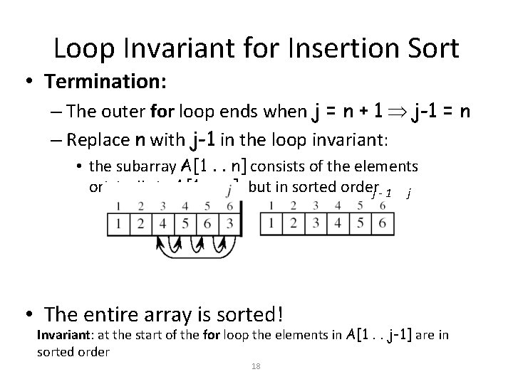
Loop Invariant for Insertion Sort • Termination: – The outer for loop ends when j = n + 1 j-1 = n – Replace n with j-1 in the loop invariant: • the subarray A[1. . n] consists of the elements originally in A[1. . n], but in sorted orderj - 1 j • The entire array is sorted! Invariant: at the start of the for loop the elements in A[1. . j-1] are in sorted order 18

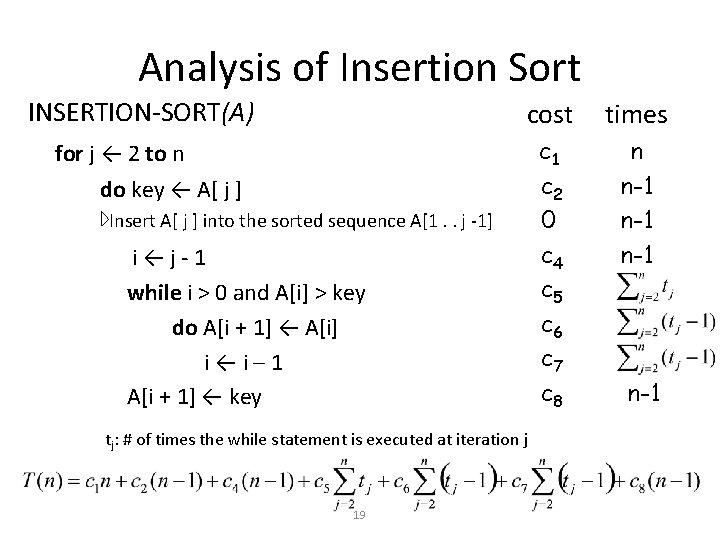
Analysis of Insertion Sort INSERTION-SORT(A) cost times c 1 c 2 0 c 4 c 5 c 6 c 7 c 8 n n-1 n-1 for j ← 2 to n do key ← A[ j ] Insert A[ j ] into the sorted sequence A[1. . j -1] i←j-1 while i > 0 and A[i] > key do A[i + 1] ← A[i] i←i– 1 A[i + 1] ← key tj: # of times the while statement is executed at iteration j 19 n-1

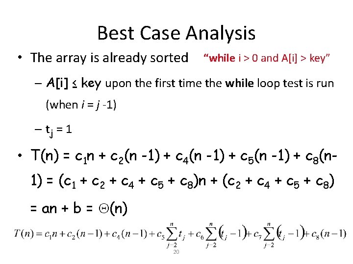
Best Case Analysis • The array is already sorted “while i > 0 and A[i] > key” – A[i] ≤ key upon the first time the while loop test is run (when i = j -1) – tj = 1 • T(n) = c 1 n + c 2(n -1) + c 4(n -1) + c 5(n -1) + c 8(n 1) = (c 1 + c 2 + c 4 + c 5 + c 8)n + (c 2 + c 4 + c 5 + c 8) = an + b = (n) 20

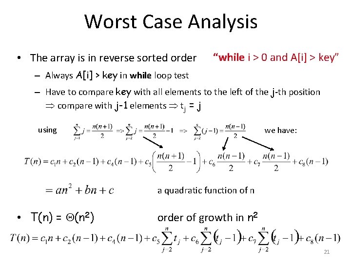
Worst Case Analysis • The array is in reverse sorted order “while i > 0 and A[i] > key” – Always A[i] > key in while loop test – Have to compare key with all elements to the left of the j-th position compare with j-1 elements tj = j using we have: a quadratic function of n • T(n) = (n 2) order of growth in n 2 21

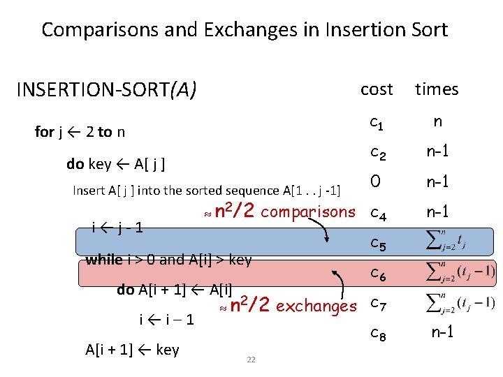
Comparisons and Exchanges in Insertion Sort INSERTION-SORT(A) for j ← 2 to n do key ← A[ j ] Insert A[ j ] into the sorted sequence A[1. . j -1] i←j-1 n 2/2 i←i– 1 A[i + 1] ← key times c 1 n c 2 n-1 0 n-1 comparisons c 4 while i > 0 and A[i] > key do A[i + 1] ← A[i] cost n 2/2 c 5 c 6 exchanges c 7 c 8 22 n-1

Insertion Sort - Summary • Advantages – Good running time for “almost sorted” arrays (n) • Disadvantages – (n 2) running time in worst and average case – n 2/2 comparisons and exchanges 23