Input Output HMMs for modeling network dynamics Sushmita

Input Output HMMs for modeling network dynamics Sushmita Roy sroy@biostat. wisc. edu Computational Network Biology Biostatistics & Medical Informatics 826 https: //compnetbiocourse. discovery. wisc. edu Oct 17 th, 18 th 2018 The style of IOHMM is adapted from Prof. Craven’s lectures on HMMs

Goals for today • What are Hidden Markov Models (HMMs)? – How do they relate to Dynamic Bayesian Networks? • What are Input/Output HMMs (IOHMMs)? • EM algorithm for learning IOHMMs • Application of IOHMMs to examine regulatory network dynamics

Motivation • Suppose we are given time series expression profiles • We wish to find key regulators that are associated with changes in expression levels over time • We have seen a simple approach to do this – Activity subgraph/skeleton network-based approaches • Can we more explicitly take time into account?

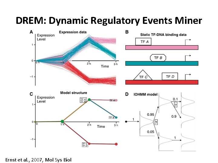
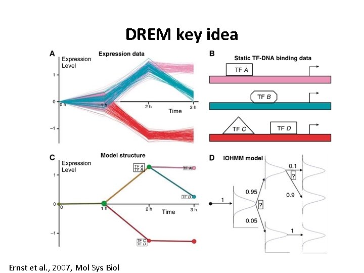
DREM: Dynamic Regulatory Events Miner Ernst et al. , 2007, Mol Sys Biol

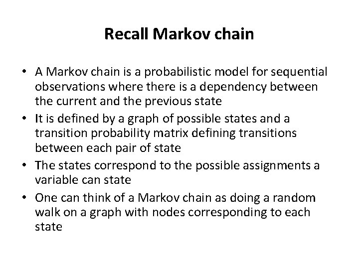
Recall Markov chain • A Markov chain is a probabilistic model for sequential observations where there is a dependency between the current and the previous state • It is defined by a graph of possible states and a transition probability matrix defining transitions between each pair of state • The states correspond to the possible assignments a variable can state • One can think of a Markov chain as doing a random walk on a graph with nodes corresponding to each state

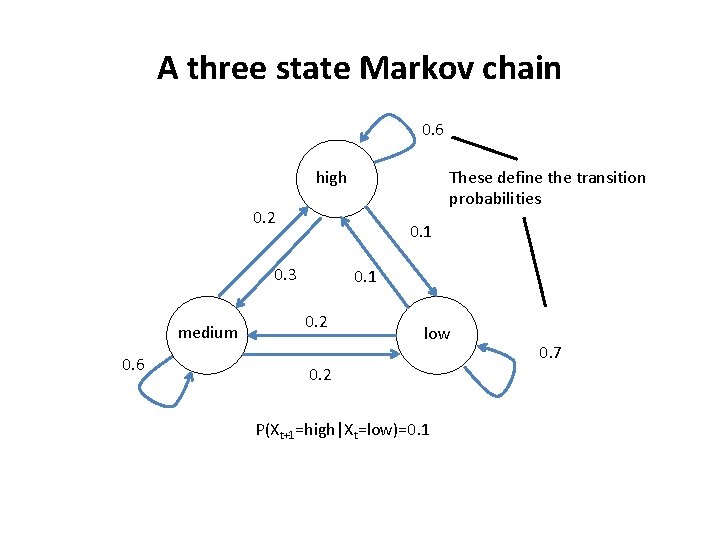
A three state Markov chain 0. 6 high These define the transition probabilities 0. 2 0. 1 0. 3 medium 0. 6 0. 1 0. 2 low 0. 2 P(Xt+1=high|Xt=low)=0. 1 0. 7

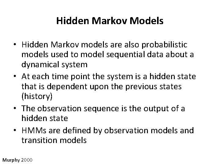
Hidden Markov Models • Hidden Markov models are also probabilistic models used to model sequential data about a dynamical system • At each time point the system is a hidden state that is dependent upon the previous states (history) • The observation sequence is the output of a hidden state • HMMs are defined by observation models and transition models Murphy 2000

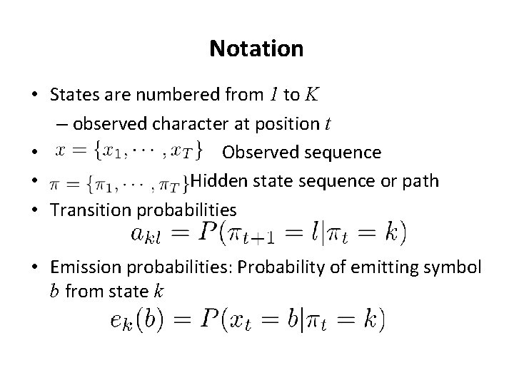
Notation • States are numbered from 1 to K – observed character at position t • Observed sequence • Hidden state sequence or path • Transition probabilities • Emission probabilities: Probability of emitting symbol b from state k

What does an HMM do? • Enables us to model observed sequences of characters generated by a hidden dynamic system • The system can exist in a fixed number of “hidden” states • The system probabilistically transitions between states and at each state it emits a symbol/character

Defining an HMM • States • Emission alphabet • Parameters – State transition probabilities for probabilistic transitions from state at time t to state at time t+1 – Emission probabilities for probabilistically emitting symbols from a state

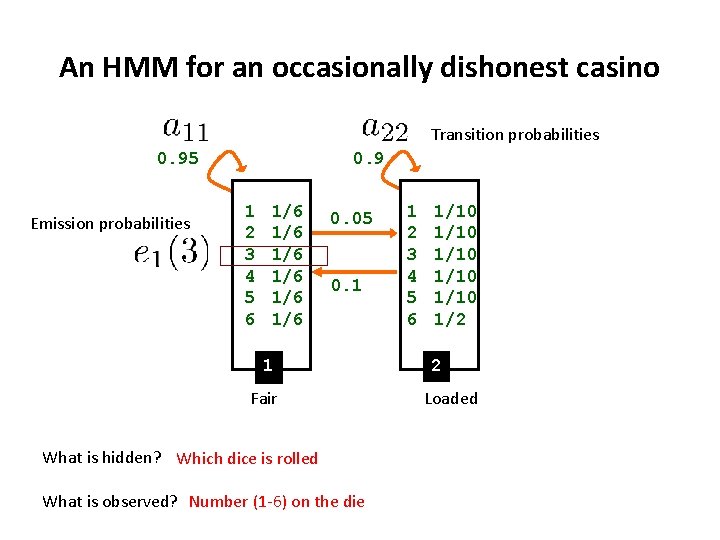
An HMM for an occasionally dishonest casino Transition probabilities 0. 95 Emission probabilities 0. 9 1 2 3 4 5 6 1/6 1/6 1/6 0. 05 0. 1 1 Fair What is hidden? Which dice is rolled What is observed? Number (1 -6) on the die 1 2 3 4 5 6 1/10 1/10 1/2 2 Loaded

Formally defining a HMM • States • Emission alphabet • Parameters – State transition probabilities for probabilistic transitions from state at time t to state at time t+1 – Emission probabilities for probabilistically emitting symbols from a state

Goals for today • What are Hidden Markov Models (HMMs)? – How do they relate to Dynamic Bayesian Networks? • What are Input/Output HMMs (IOHMMs)? • Learning problems of IOHMMs • Application of IOHMMs to examine regulatory network dynamics

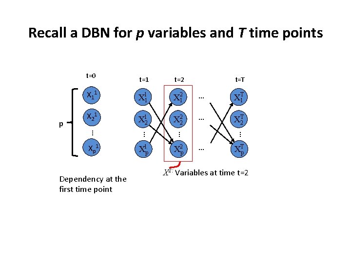
Recall a DBN for p variables and T time points t=0 p X 21 … XT 1 X 21 X 12 X 22 … XTp Dependency at the first time point X 1 p X 2 p … X 11 Xp 1 t=T … X 11 … t=2 … t=1 X 2: Variables at time t=2

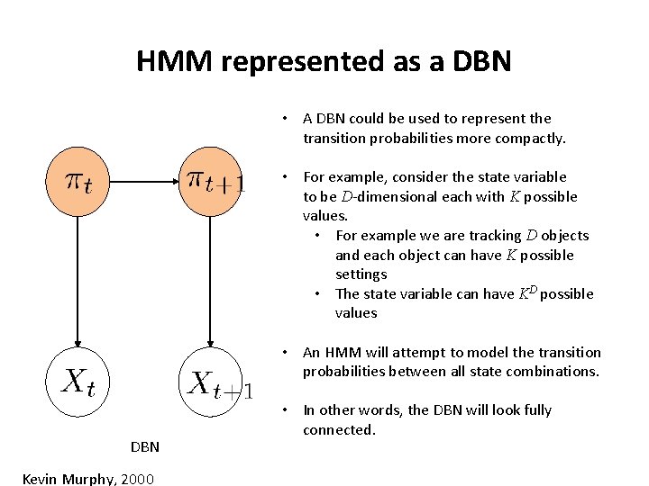
HMM represented as a DBN • A DBN could be used to represent the transition probabilities more compactly. • For example, consider the state variable to be D-dimensional each with K possible values. • For example we are tracking D objects and each object can have K possible settings • The state variable can have KD possible values • An HMM will attempt to model the transition probabilities between all state combinations. DBN Kevin Murphy, 2000 • In other words, the DBN will look fully connected.

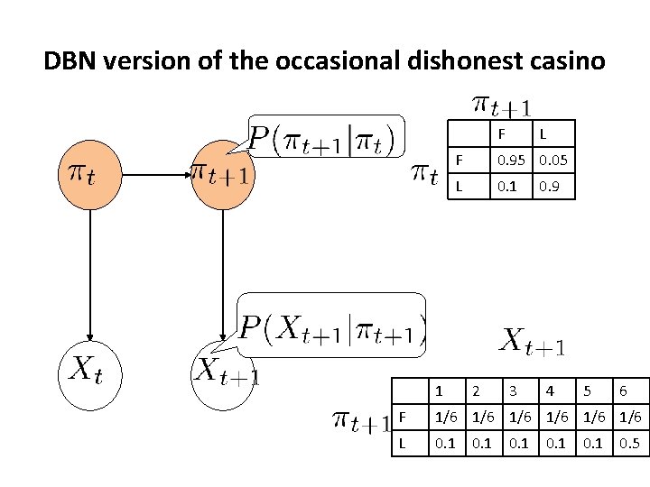
DBN version of the occasional dishonest casino F L F 0. 95 0. 05 L 0. 1 1 2 3 0. 9 4 5 6 F 1/6 1/6 1/6 L 0. 1 0. 5

Three important questions in HMMs • What is the probability of a sequence from an HMM? – Forward algorithm • What is the most likely sequence of states for generating a sequence of observations – Viterbi algorithm • How can we learn an HMM from a set of sequences? – Forward-backward or Baum-Welch (an EM algorithm)

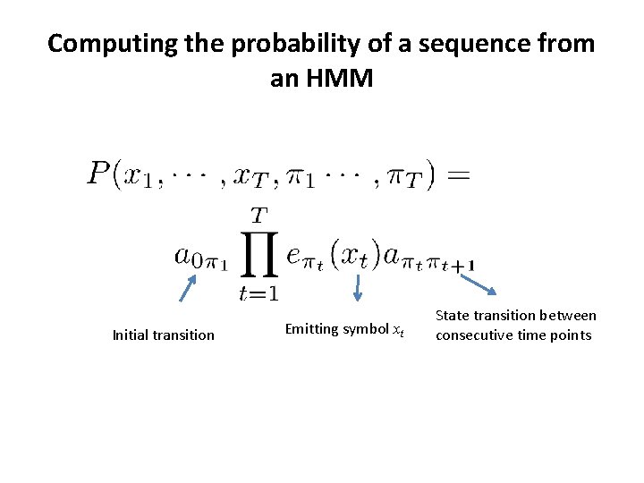
Computing the probability of a sequence from an HMM Initial transition Emitting symbol xt State transition between consecutive time points

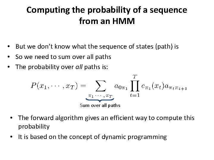
Computing the probability of a sequence from an HMM • But we don’t know what the sequence of states (path) is • So we need to sum over all paths • The probability over all paths is: Sum over all paths • The forward algorithm gives an efficient way to compute this probability • It is based on the concept of dynamic programming

Goals for today • What are Hidden Markov Models (HMMs)? – How do they relate to Dynamic Bayesian Networks? • What are Input/Output HMMs (IOHMMs)? • Learning problems of IOHMMs • Application of IOHMMs to examine regulatory network dynamics

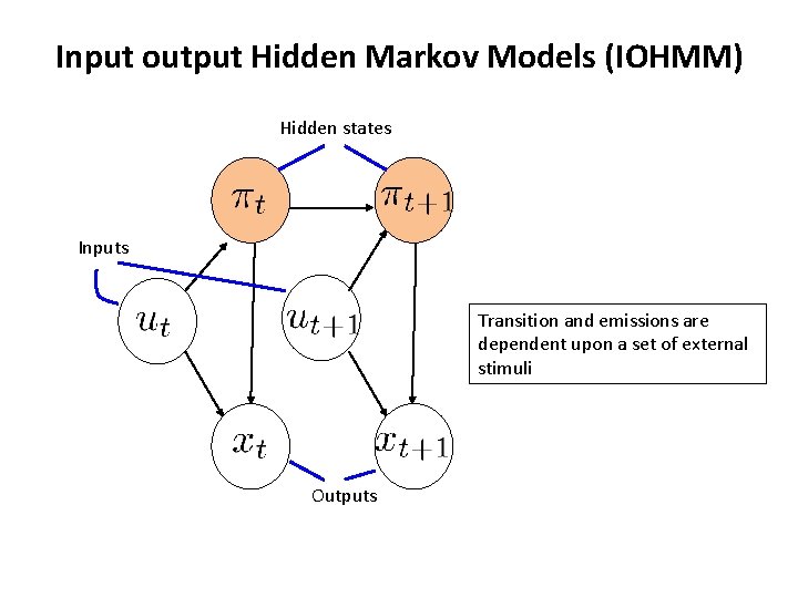
Input output Hidden Markov Models (IOHMM) • As in the HMM we have – States, emissions and transitions • In addition we have a sequence of inputs – The transitions and emissions can depend on inputs (u 1, . . , u. T) • In a way, IOHMMs map inputs to outputs – This is different from HMMs • HMMs aim to define P(x 1. . x. T) while IOHMMs define P(x 1. . x. T|u 1. . u. T) Bengio & Frasconi, IEEE Trans on Neural Networks 1996

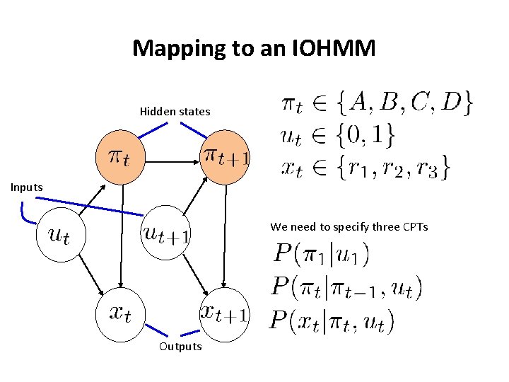
Input output Hidden Markov Models (IOHMM) Hidden states Inputs Transition and emissions are dependent upon a set of external stimuli Outputs

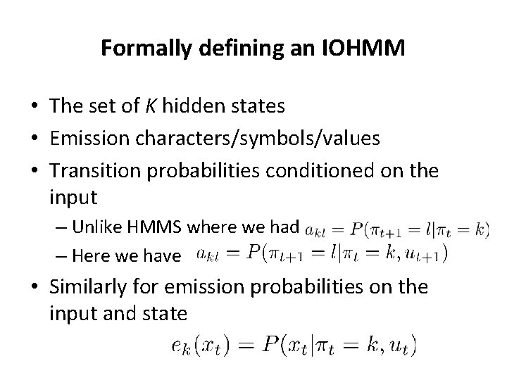
Formally defining an IOHMM • The set of K hidden states • Emission characters/symbols/values • Transition probabilities conditioned on the input – Unlike HMMS where we had – Here we have • Similarly for emission probabilities on the input and state

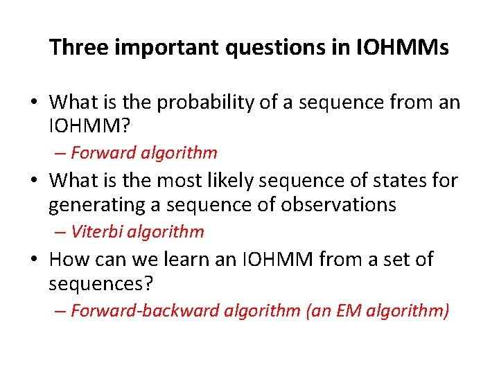
Three important questions in IOHMMs • What is the probability of a sequence from an IOHMM? – Forward algorithm • What is the most likely sequence of states for generating a sequence of observations – Viterbi algorithm • How can we learn an IOHMM from a set of sequences? – Forward-backward algorithm (an EM algorithm)

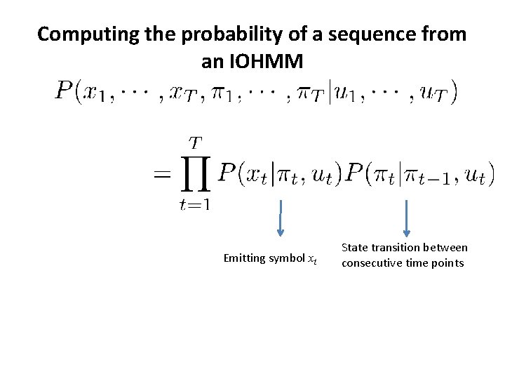
Computing the probability of a sequence from an IOHMM Emitting symbol xt State transition between consecutive time points

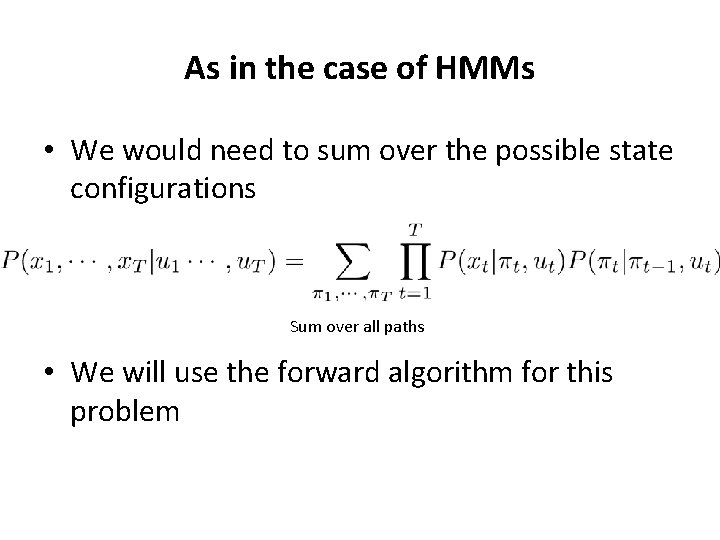
As in the case of HMMs • We would need to sum over the possible state configurations Sum over all paths • We will use the forward algorithm for this problem

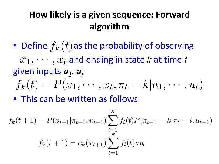
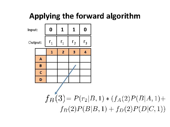
How likely is a given sequence: Forward algorithm • Define as the probability of observing and ending in state k at time t given inputs u 1. . ut • This can be written as follows

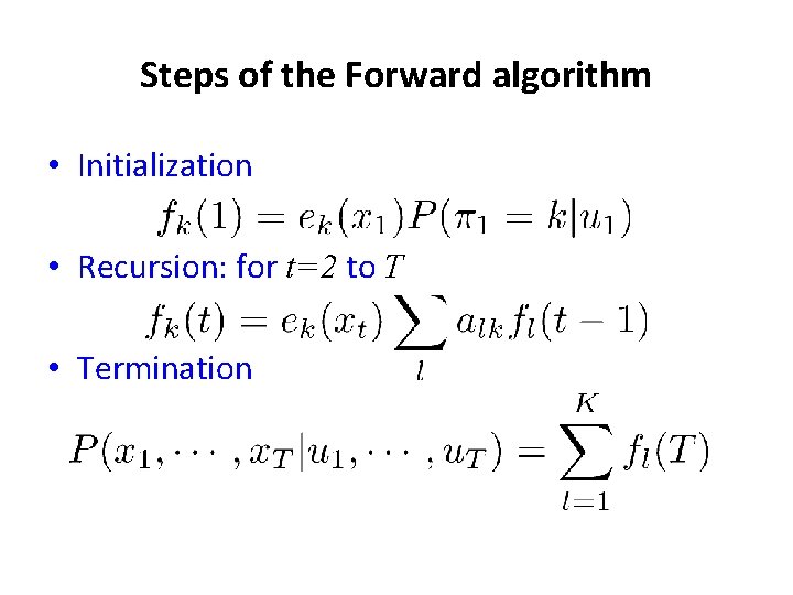
Steps of the Forward algorithm • Initialization • Recursion: for t=2 to T • Termination

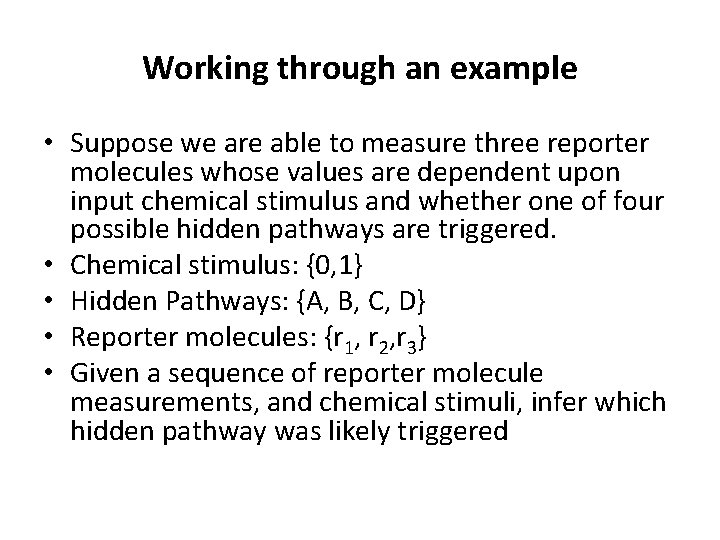
Working through an example • Suppose we are able to measure three reporter molecules whose values are dependent upon input chemical stimulus and whether one of four possible hidden pathways are triggered. • Chemical stimulus: {0, 1} • Hidden Pathways: {A, B, C, D} • Reporter molecules: {r 1, r 2, r 3} • Given a sequence of reporter molecule measurements, and chemical stimuli, infer which hidden pathway was likely triggered

Mapping to an IOHMM Hidden states Inputs We need to specify three CPTs Outputs

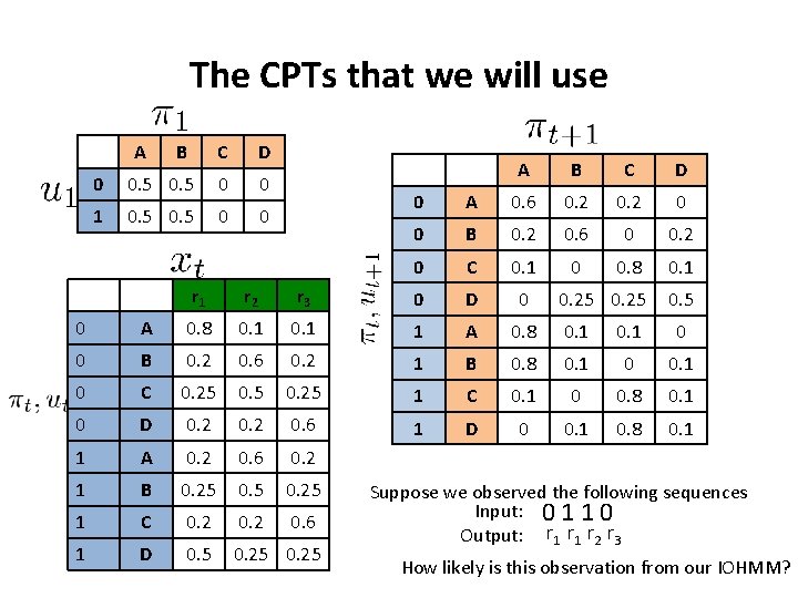
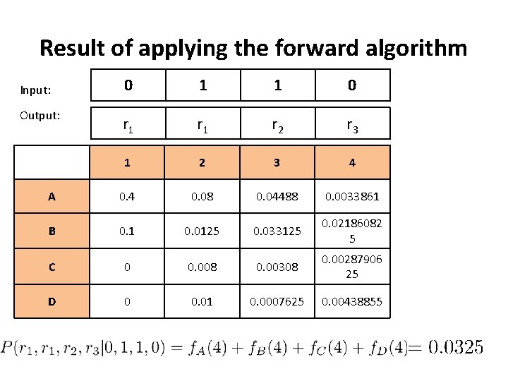
The CPTs that we will use A B C D 0 0. 5 0 0 1 0. 5 0 0 A B C D 0 A 0. 6 0. 2 0 0 B 0. 2 0. 6 0 0. 2 0 C 0. 1 0 0. 8 0. 1 0. 25 0. 5 r 1 r 2 r 3 0 D 0 0 A 0. 8 0. 1 1 A 0. 8 0. 1 0 0 B 0. 2 0. 6 0. 2 1 B 0. 8 0. 1 0 C 0. 25 1 C 0. 1 0 0. 8 0. 1 0 D 0. 2 0. 6 1 D 0 0. 1 0. 8 0. 1 1 A 0. 2 0. 6 0. 2 1 B 0. 25 1 C 0. 2 0. 6 1 D 0. 5 0. 25 Suppose we observed the following sequences Input: 0 1 1 0 Output: r 1 r 2 r 3 How likely is this observation from our IOHMM?

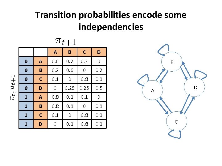
Transition probabilities encode some independencies A B C D 0 A 0. 6 0. 2 0 0 B 0. 2 0. 6 0 0. 2 0 C 0. 1 0 0. 8 0. 1 0 D 0 0. 25 0. 5 1 A 0. 8 0. 1 0 1 B 0. 8 0. 1 0 0. 1 1 C 0. 1 0 0. 8 0. 1 1 D 0 0. 1 0. 8 0. 1 B D A C

Applying the forward algorithm Input: 0 1 1 0 Output: r 1 r 2 r 3 1 2 3 4 A B C D

Result of applying the forward algorithm 0 1 1 0 r 1 r 2 r 3 1 2 3 4 A 0. 4 0. 08 0. 04488 0. 0033861 B 0. 1 0. 0125 0. 033125 0. 02186082 5 C 0 0. 008 0. 00308 0. 00287906 25 D 0 0. 01 0. 0007625 0. 00438855 Input: Output:

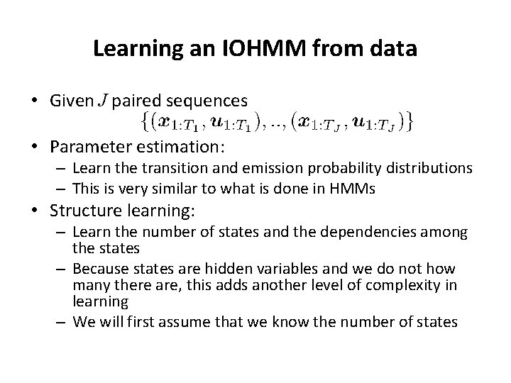
Learning an IOHMM from data • Given J paired sequences • Parameter estimation: – Learn the transition and emission probability distributions – This is very similar to what is done in HMMs • Structure learning: – Learn the number of states and the dependencies among the states – Because states are hidden variables and we do not how many there are, this adds another level of complexity in learning – We will first assume that we know the number of states

The expectation maximization algorithm • Expectation Maximization (EM) is a widely used when there are hidden variables • It is an iterative algorithm that maximizes the likelihood of the data • Each iteration is made up of two steps – Expectation step (E): estimate the expected values of hidden variables given the data and previous parameter settings – Maximization step (M): estimate the parameters using the expected counts

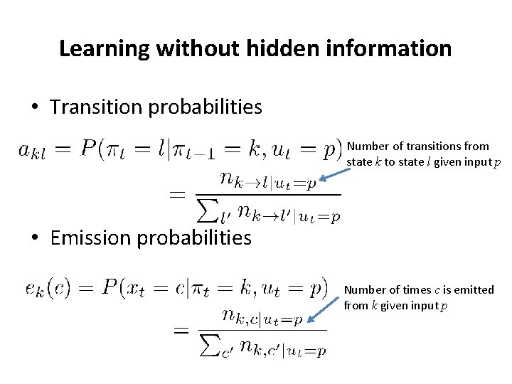
Learning without hidden information • Transition probabilities Number of transitions from state k to state l given input p • Emission probabilities Number of times c is emitted from k given input p

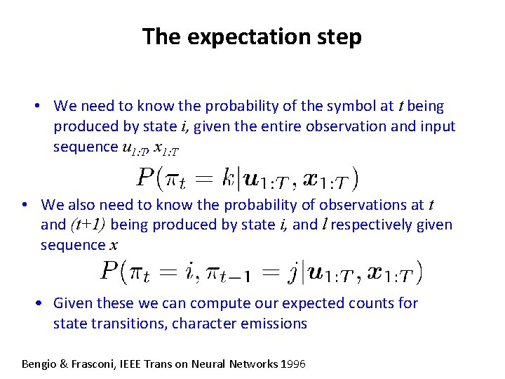
The expectation step • We need to know the probability of the symbol at t being produced by state i, given the entire observation and input sequence u 1: T, x 1: T • We also need to know the probability of observations at t and (t+1) being produced by state i, and l respectively given sequence x • Given these we can compute our expected counts for state transitions, character emissions Bengio & Frasconi, IEEE Trans on Neural Networks 1996

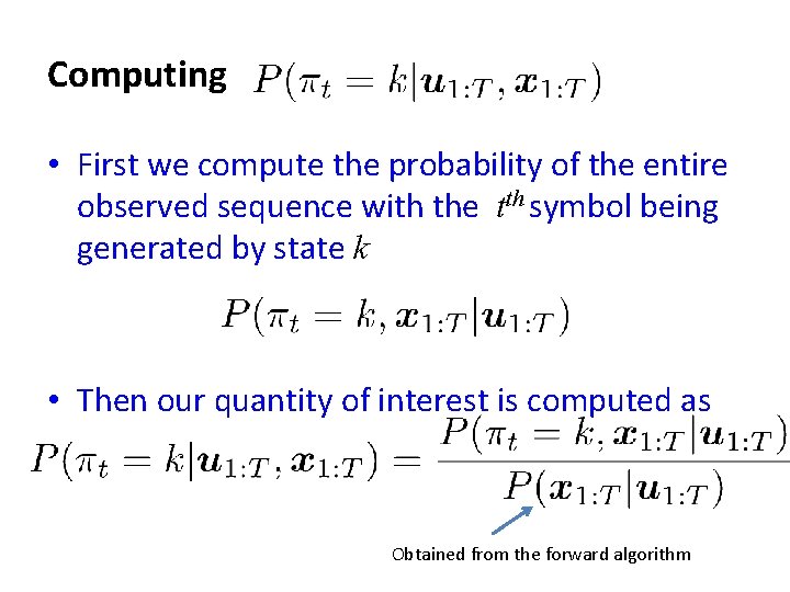
Computing • First we compute the probability of the entire observed sequence with the tth symbol being generated by state k • Then our quantity of interest is computed as Obtained from the forward algorithm

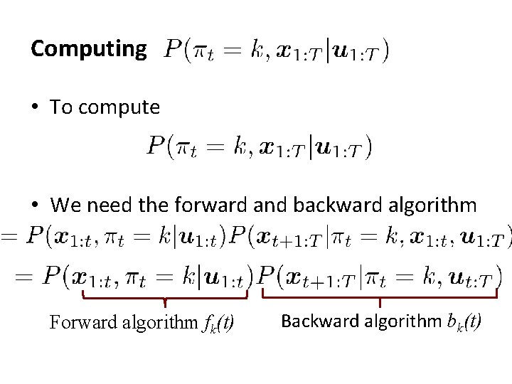
Computing • To compute • We need the forward and backward algorithm Forward algorithm fk(t) Backward algorithm bk(t)

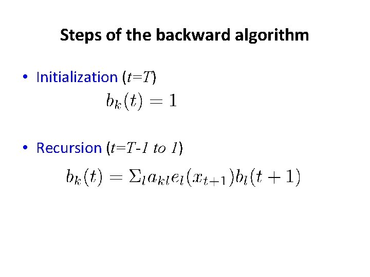
Steps of the backward algorithm • Initialization (t=T) • Recursion (t=T-1 to 1)

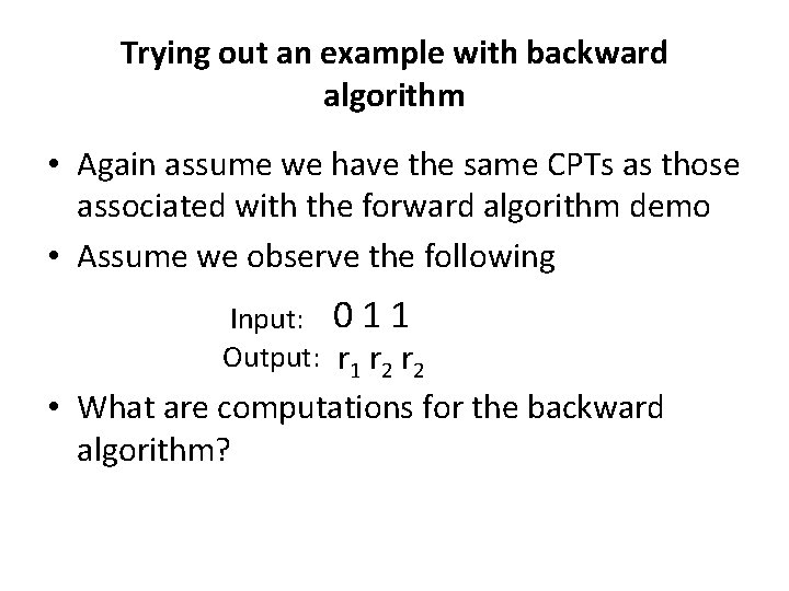
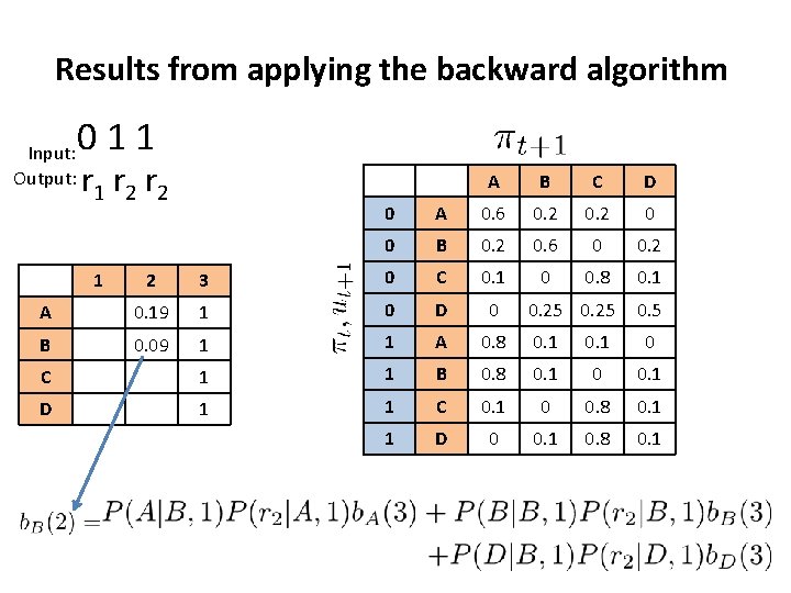
Trying out an example with backward algorithm • Again assume we have the same CPTs as those associated with the forward algorithm demo • Assume we observe the following Input: 0 1 1 Output: r 1 r 2 • What are computations for the backward algorithm?

Results from applying the backward algorithm Input: Output: 011 r 2 r 2 A B C D 0 A 0. 6 0. 2 0 0 B 0. 2 0. 6 0 0. 2 0 0. 8 0. 1 0. 25 0. 5 2 3 0 C 0. 1 A 0. 19 1 0 D 0 B 0. 09 1 1 A 0. 8 0. 1 0 C 1 1 B 0. 8 0. 1 0 0. 1 D 1 1 C 0. 1 0 0. 8 0. 1 1 D 0 0. 1 0. 8 0. 1 1

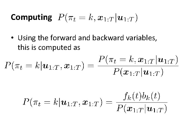
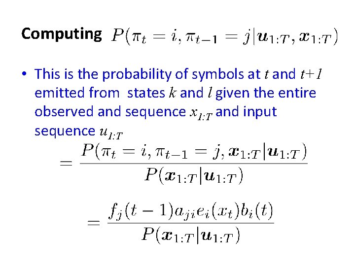
Computing • Using the forward and backward variables, this is computed as

Computing • This is the probability of symbols at t and t+1 emitted from states k and l given the entire observed and sequence x 1: T and input sequence u 1: T

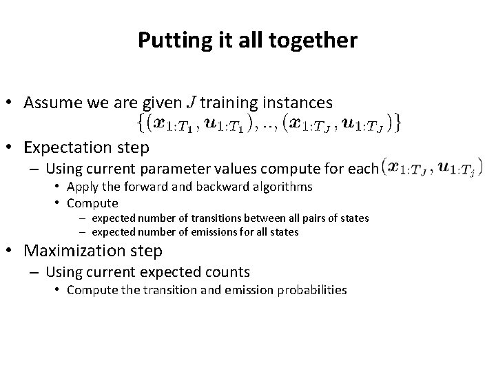
Putting it all together • Assume we are given J training instances • Expectation step – Using current parameter values compute for each • Apply the forward and backward algorithms • Compute – expected number of transitions between all pairs of states – expected number of emissions for all states • Maximization step – Using current expected counts • Compute the transition and emission probabilities

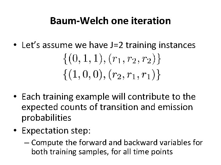
Baum-Welch one iteration • Let’s assume we have J=2 training instances • Each training example will contribute to the expected counts of transition and emission probabilities • Expectation step: – Compute the forward and backward variables for both training samples, for all time points

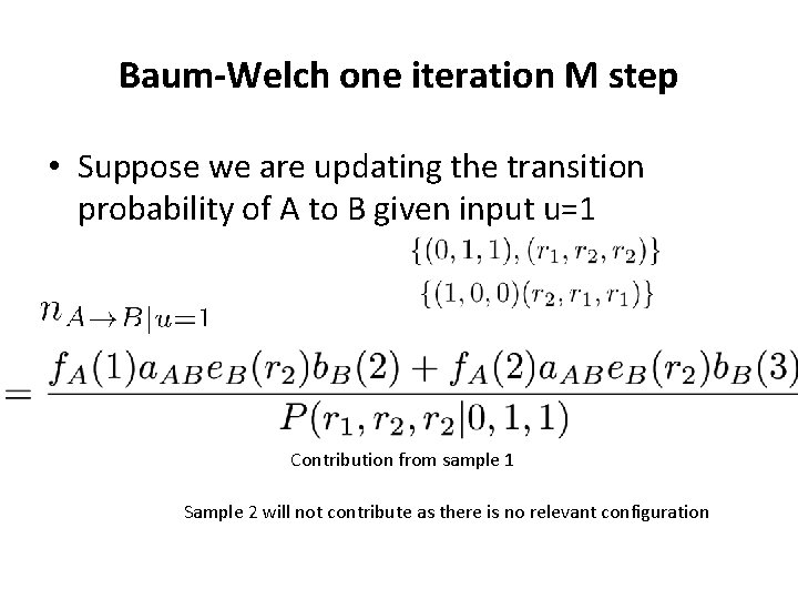
Baum-Welch one iteration M step • Suppose we are updating the transition probability of A to B given input u=1 Contribution from sample 1 Sample 2 will not contribute as there is no relevant configuration

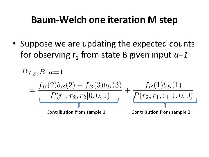
Baum-Welch one iteration M step • Suppose we are updating the expected counts for observing r 2 from state B given input u=1 Contribution from sample 2

Goals for today • What are Hidden Markov Models (HMMs)? – How do they relate to Dynamic Bayesian Networks? • What are Input/Output HMMs (IOHMMs)? • Learning problems of IOHMMs • Application of IOHMMs to examine regulatory network dynamics

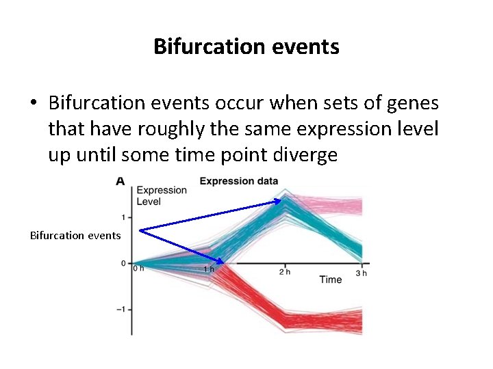
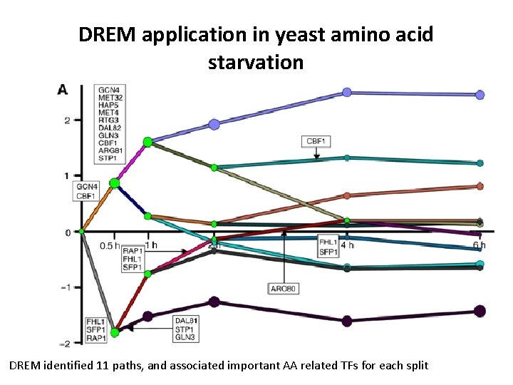
Bifurcation events • Bifurcation events occur when sets of genes that have roughly the same expression level up until some time point diverge Bifurcation events

Dynamic Regulatory Events Miner (DREM) • Given – a gene expression time course – Static TF binding data or signaling networks • Do – Identifies important regulators for interesting temporal changes • DREM is suited for short time courses • DREM is based on an Input-Output HMM Ernst et al. , 2007 Mol Sys Biol

DREM key idea Ernst et al. , 2007, Mol Sys Biol

IOHMM model in DREM • The output distributions were modeled as Gaussians – Enabled modeling continuous expression values • State transitions depended on static input and the current state – A binary classifier was trained in the M step for each state with two children, to discriminate between genes assigned to the bifurcating states

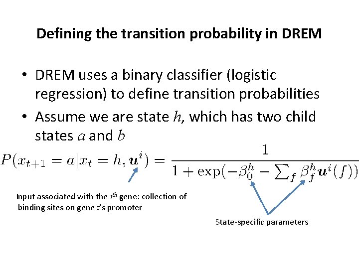
Defining the transition probability in DREM • DREM uses a binary classifier (logistic regression) to define transition probabilities • Assume we are state h, which has two child states a and b Input associated with the ith gene: collection of binding sites on gene i’s promoter State-specific parameters

Results • Application of DREM to yeast expression data – Amino acid (AA) starvation – One time point Ch. IP binding in AA starvation • Analysis of condition-specific binding • Application to multiple stress and normal conditions

DREM application in yeast amino acid starvation DREM identified 11 paths, and associated important AA related TFs for each split

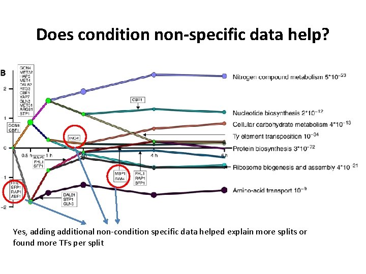
Does condition non-specific data help? Yes, adding additional non-condition specific data helped explain more splits or found more TFs per split

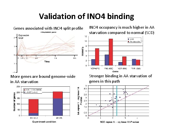
Validation of INO 4 binding • INO 4 was a novel prediction by the method • Using a small scale experiment, test binding in 4 gene promoters after AA starvation • Measure genome-wide binding profile of INO 4 in AA starvation and SCD and compare relative binding

Validation of INO 4 binding Genes associated with INO 4 split profile More genes are bound genome-wide in AA starvation INO 4 occupancy is much higher in AA starvation compared to normal (SCD) Stronger binding in AA starvation of genes in this path

Does integration help? • Randomize Ch. IP data and ask if enriched TFs with paths were identified – Fewer TFs were identified • Compare IOHMM vs HMM – Lesser enrichment of Gene Ontology processes in HMMs paths compared to IOHMMs

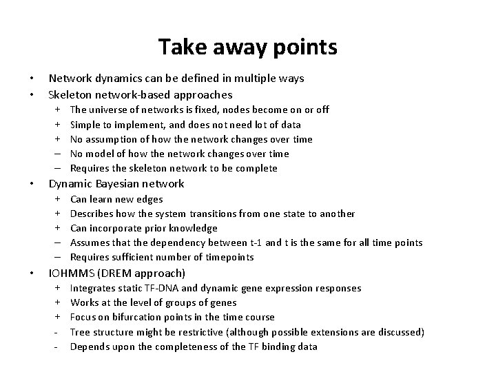
Take away points • • Network dynamics can be defined in multiple ways Skeleton network-based approaches + + + – – • Dynamic Bayesian network + + + – – • The universe of networks is fixed, nodes become on or off Simple to implement, and does not need lot of data No assumption of how the network changes over time No model of how the network changes over time Requires the skeleton network to be complete Can learn new edges Describes how the system transitions from one state to another Can incorporate prior knowledge Assumes that the dependency between t-1 and t is the same for all time points Requires sufficient number of timepoints IOHMMS (DREM approach) + + + - Integrates static TF-DNA and dynamic gene expression responses Works at the level of groups of genes Focus on bifurcation points in the time course Tree structure might be restrictive (although possible extensions are discussed) Depends upon the completeness of the TF binding data