Initial fluctuations and anisotropies in heavy ion collisions

Initial fluctuations and anisotropies in heavy ion collisions Cyrille Marquet Centre de Physique Théorique École Polytechnique & CNRS based on: Albacete, Guerrero-Rodriguez, CM, JHEP 1901 (2019) 073 Giacalone, Guerrero-Rodriguez, Luzum, CM and Ollitrault, ar. Xiv: 1902. 07168

Outline • The fluid paradigm final-state momentum anisotropies from initial-state spatial anisotropies • Initial eccentricities from the Glasma how to calculate the initial spatial anisotropies: from the energy momentum tensor and its fluctuations • A new picture ab-initio description free from the Monte Carlo Glauber Ansatz

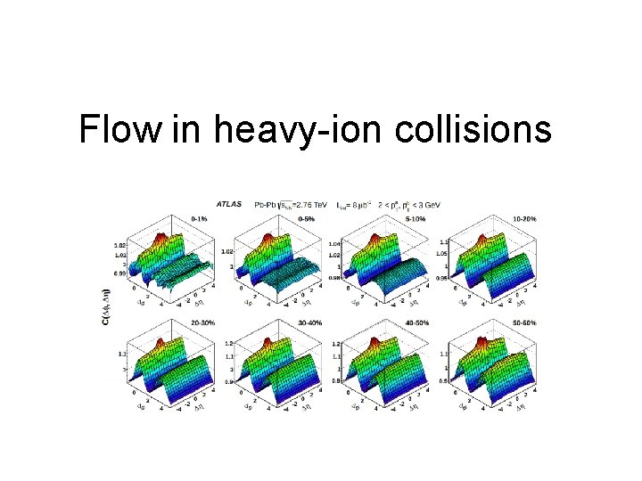
Flow in heavy-ion collisions

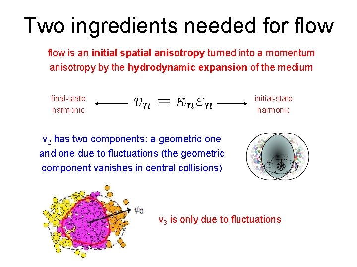
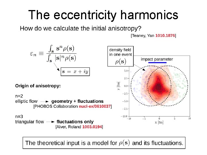
Two ingredients needed for flow is an initial spatial anisotropy turned into a momentum anisotropy by the hydrodynamic expansion of the medium final-state harmonic initial-state harmonic v 2 has two components: a geometric one and one due to fluctuations (the geometric component vanishes in central collisions) v 3 is only due to fluctuations

The eccentricity harmonics

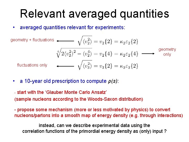
Relevant averaged quantities • averaged quantities relevant for experiments: geometry + fluctuations geometry only fluctuations only • a 10 -year old prescription to compute ρ(s): - start with the ‘Glauber Monte Carlo Ansatz’ (sample nucleons according to the Woods-Saxon distribution) - propose some mechanism (more or less motivated by physics) to convert nucleons/partons into a smooth map of energy density (e. g. through interactions) instead, can we describe experimental data using the correlation functions of the primordial energy density as (only) input ?

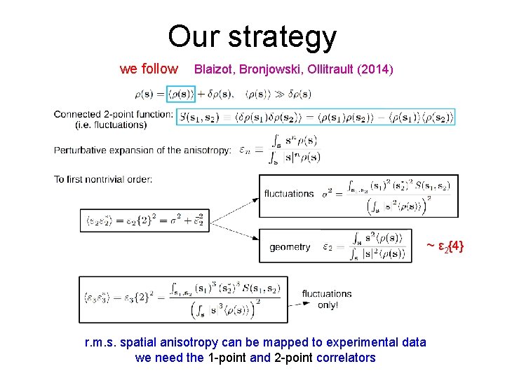
Our strategy we follow Blaizot, Bronjowski, Ollitrault (2014) ~ ε 2{4} r. m. s. spatial anisotropy can be mapped to experimental data we need the 1 -point and 2 -point correlators

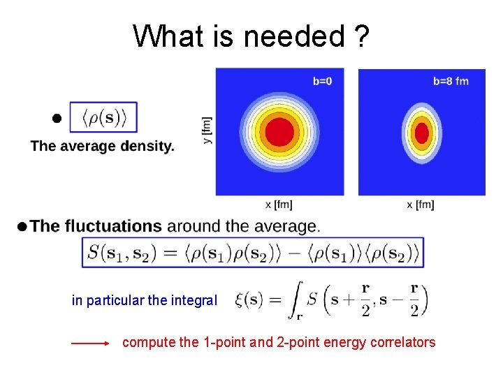
What is needed ? in particular the integral compute the 1 -point and 2 -point energy correlators

Initial eccentricities from the Glasma Albacete, Guerrero-Rodriguez, CM, JHEP 1901 (2019) 073

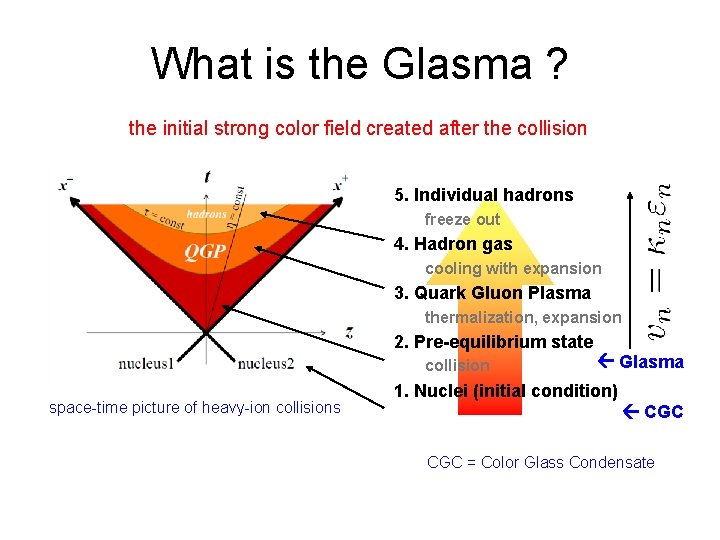
What is the Glasma ? the initial strong color field created after the collision 5. Individual hadrons freeze out 4. Hadron gas cooling with expansion 3. Quark Gluon Plasma thermalization, expansion 2. Pre-equilibrium state collision space-time picture of heavy-ion collisions Glasma 1. Nuclei (initial condition) CGC = Color Glass Condensate

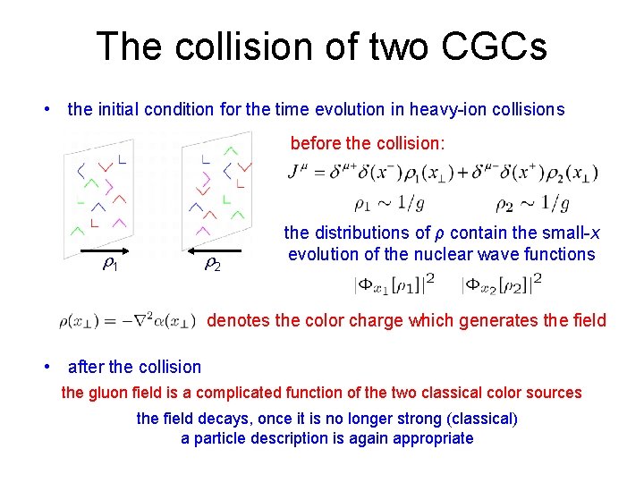
The collision of two CGCs • the initial condition for the time evolution in heavy-ion collisions before the collision: r 1 r 2 the distributions of ρ contain the small-x evolution of the nuclear wave functions denotes the color charge which generates the field • after the collision the gluon field is a complicated function of the two classical color sources the field decays, once it is no longer strong (classical) a particle description is again appropriate

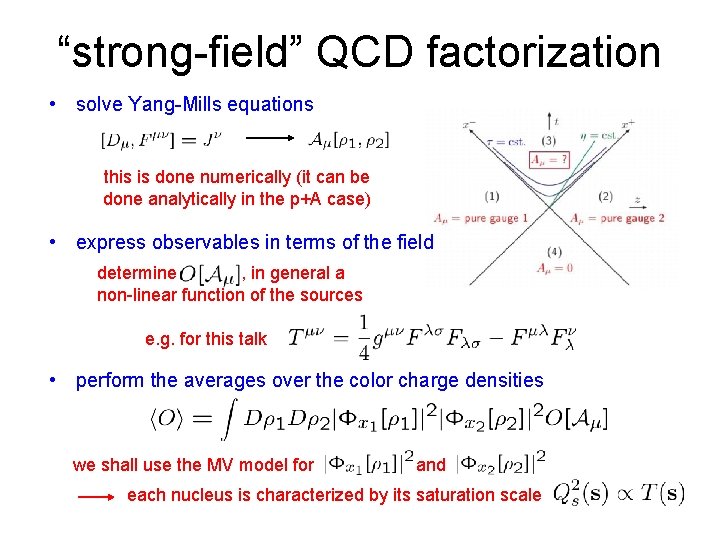
“strong-field” QCD factorization • solve Yang-Mills equations this is done numerically (it can be done analytically in the p+A case) • express observables in terms of the field determine , in general a non-linear function of the sources e. g. for this talk • perform the averages over the color charge densities we shall use the MV model for and each nucleus is characterized by its saturation scale

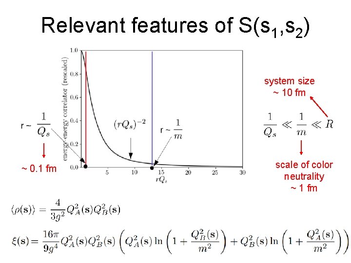
Relevant features of S(s 1, s 2) system size ~ 10 fm ~ 0. 1 fm scale of color neutrality ~ 1 fm

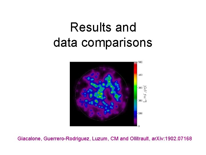
Results and data comparisons Giacalone, Guerrero-Rodriguez, Luzum, CM and Ollitrault, ar. Xiv: 1902. 07168

Comparison to MC Glauber models mean anisotropy rms ε 2 fluctuations rms ε 3 IP Glasma ~ MC Glauber, their fluctuations are dominated by the nucleon position sampling we only have fluctuations of the local color charge

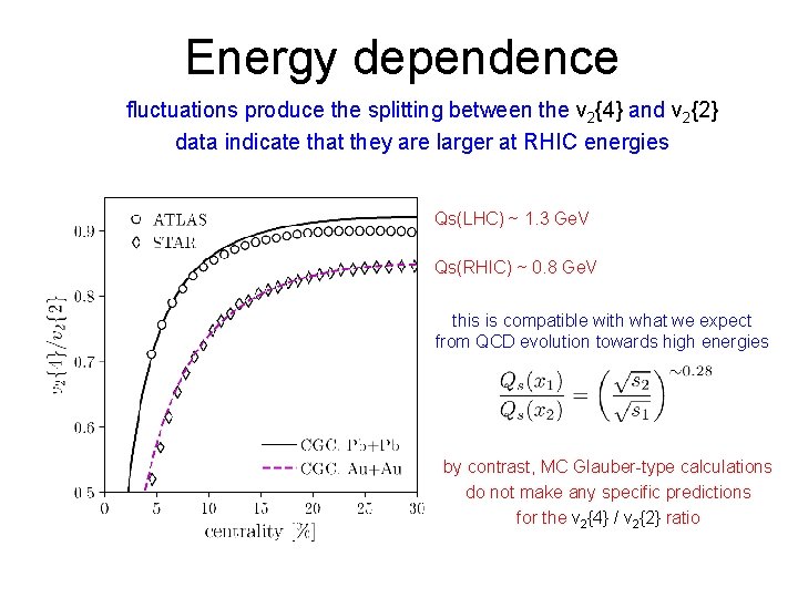
Comparison to data - v 2{4} simply probes the average geometry, we use it to fix κ 2 - then, with a reasonable Qs value, we can reproduce the fluctuations in v 2{2} - the response coefficients are compatible with state-of-the-art hydro simulations - Qs(LHC) > Qs(RHIC) explains more eccentricity fluctuations at RHIC

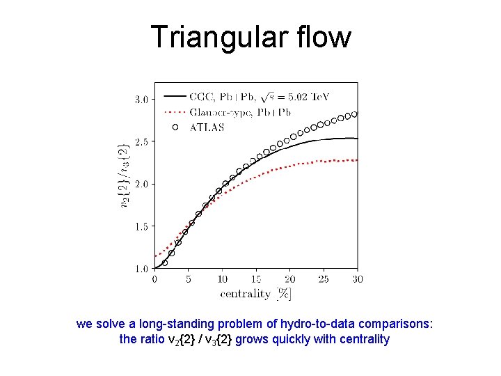
Triangular flow we solve a long-standing problem of hydro-to-data comparisons: the ratio v 2{2} / v 3{2} grows quickly with centrality

Energy dependence fluctuations produce the splitting between the v 2{4} and v 2{2} data indicate that they are larger at RHIC energies Qs(LHC) ~ 1. 3 Ge. V Qs(RHIC) ~ 0. 8 Ge. V this is compatible with what we expect from QCD evolution towards high energies by contrast, MC Glauber-type calculations do not make any specific predictions for the v 2{4} / v 2{2} ratio

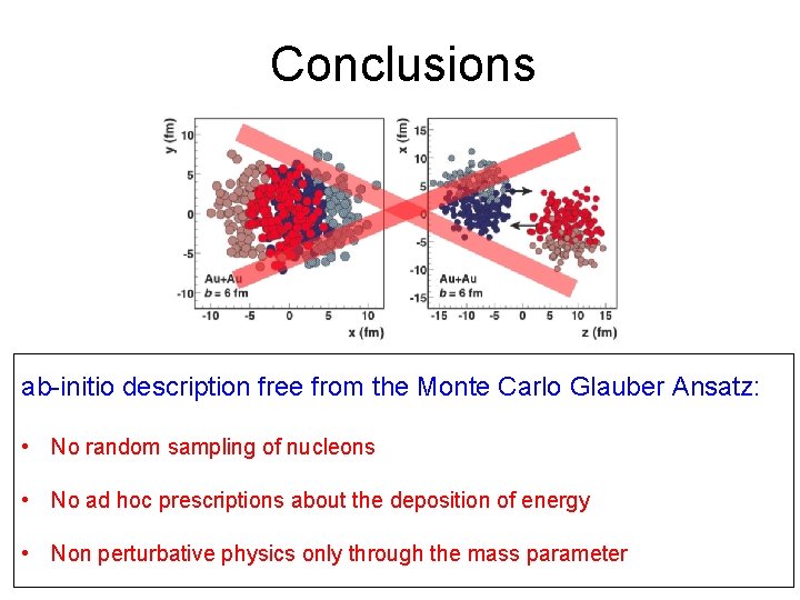
Conclusions ab-initio description free from the Monte Carlo Glauber Ansatz: • No random sampling of nucleons • No ad hoc prescriptions about the deposition of energy • Non perturbative physics only through the mass parameter