Information Retrieval Models Language Models Cheng Xiang Zhai

Information Retrieval Models: Language Models Cheng. Xiang Zhai Department of Computer Science University of Illinois, Urbana-Champaign

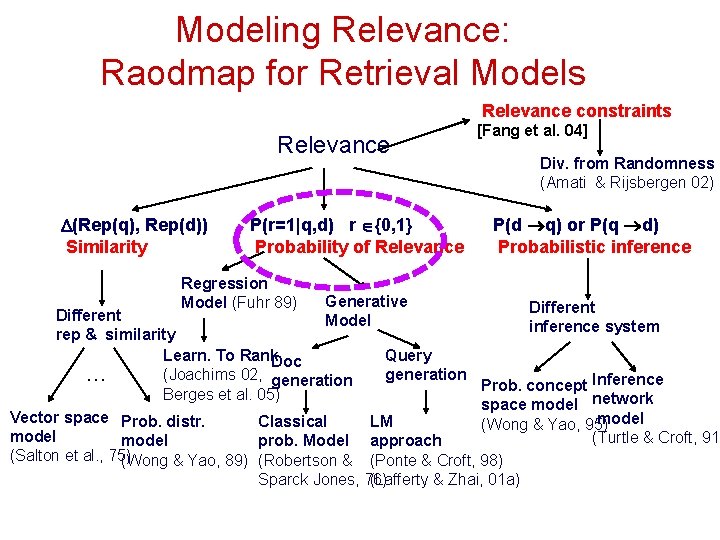
Modeling Relevance: Raodmap for Retrieval Models Relevance constraints Relevance (Rep(q), Rep(d)) Similarity P(r=1|q, d) r {0, 1} Probability of Relevance Regression Model (Fuhr 89) Generative Model [Fang et al. 04] Div. from Randomness (Amati & Rijsbergen 02) P(d q) or P(q d) Probabilistic inference Different inference system rep & similarity Learn. To Rank. Doc Query (Joachims 02, generation … Prob. concept Inference Berges et al. 05) space model network Vector space Prob. distr. model Classical LM (Wong & Yao, 95) model (Turtle & Croft, 91) model prob. Model approach (Salton et al. , 75) (Wong & Yao, 89) (Robertson & (Ponte & Croft, 98) Sparck Jones, 76) (Lafferty & Zhai, 01 a)

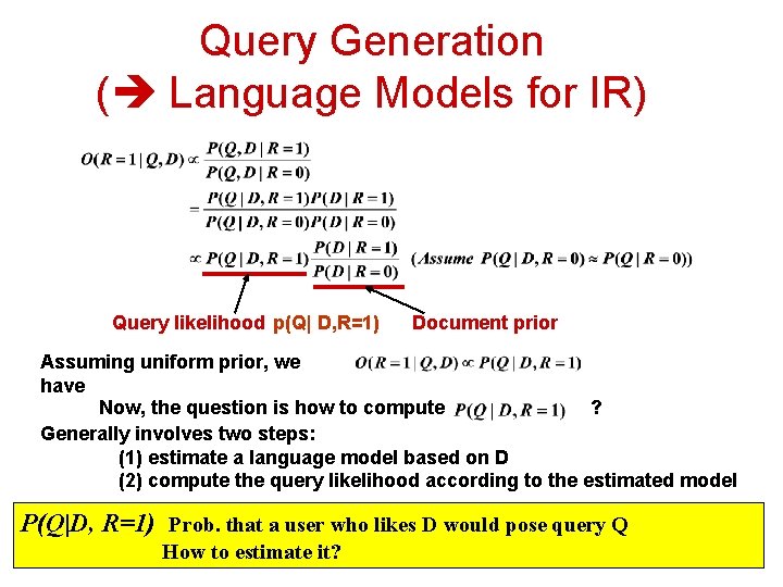
Query Generation ( Language Models for IR) Query likelihood p(Q| D, R=1) Document prior Assuming uniform prior, we have Now, the question is how to compute ? Generally involves two steps: (1) estimate a language model based on D (2) compute the query likelihood according to the estimated model P(Q|D, R=1) Prob. that a user who likes D would pose query Q How to estimate it?

The Basic LM Approach [Ponte & Croft 98] Document Language Model … Text mining paper text ? mining ? assocation ? clustering ? … food ? … Food nutrition paper … food ? nutrition ? healthy ? diet ? … Query = “data mining algorithms” ? Which model would most likely have generated this query?

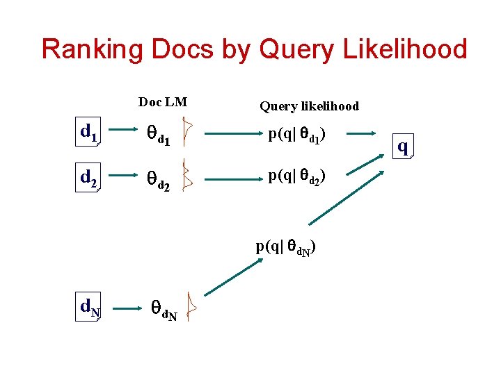
Ranking Docs by Query Likelihood Doc LM Query likelihood d 1 p(q| d 1) d 2 p(q| d 2) p(q| d. N) d. N q

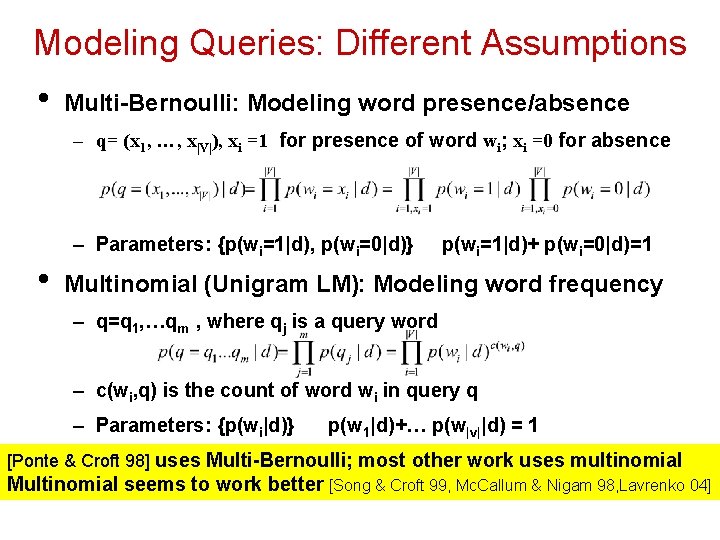
Modeling Queries: Different Assumptions • Multi-Bernoulli: Modeling word presence/absence – q= (x 1, …, x|V|), xi =1 for presence of word wi; xi =0 for absence • – Parameters: {p(wi=1|d), p(wi=0|d)} p(wi=1|d)+ p(wi=0|d)=1 Multinomial (Unigram LM): Modeling word frequency – q=q 1, …qm , where qj is a query word – c(wi, q) is the count of word wi in query q – Parameters: {p(wi|d)} p(w 1|d)+… p(w|v||d) = 1 [Ponte & Croft 98] uses Multi-Bernoulli; most other work uses multinomial Multinomial seems to work better [Song & Croft 99, Mc. Callum & Nigam 98, Lavrenko 04]

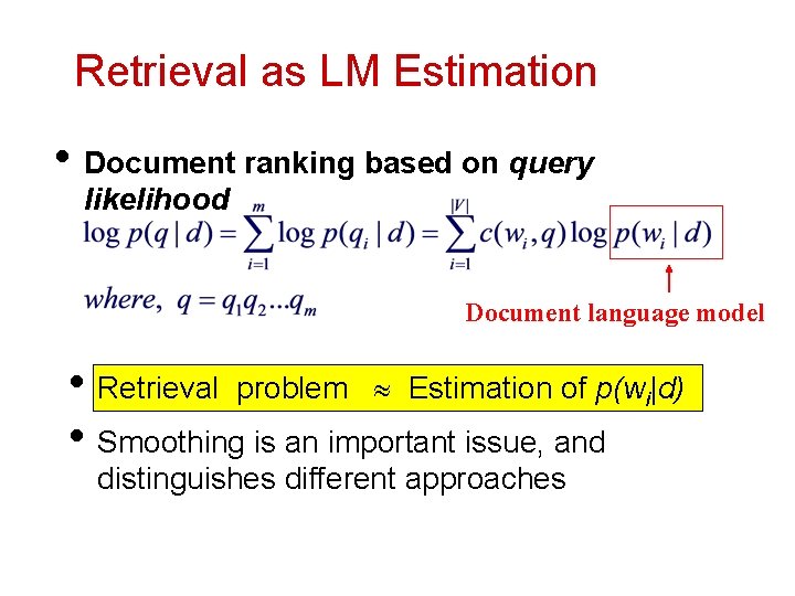
Retrieval as LM Estimation • Document ranking based on query likelihood Document language model • Retrieval problem Estimation of p(wi|d) • Smoothing is an important issue, and distinguishes different approaches

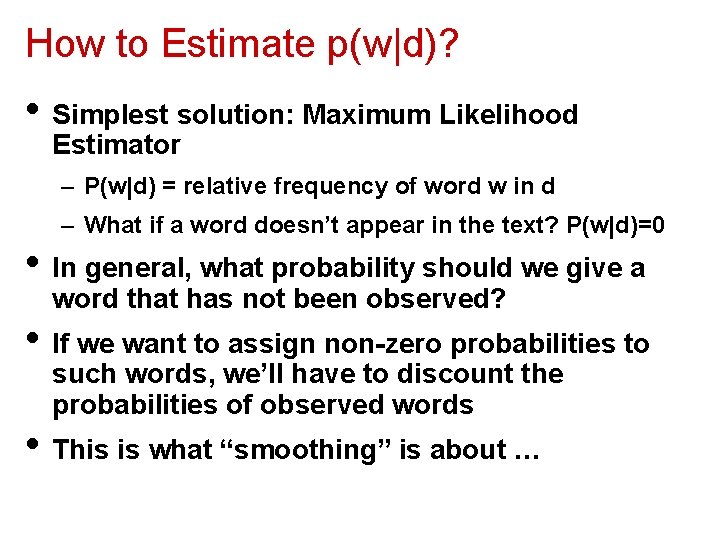
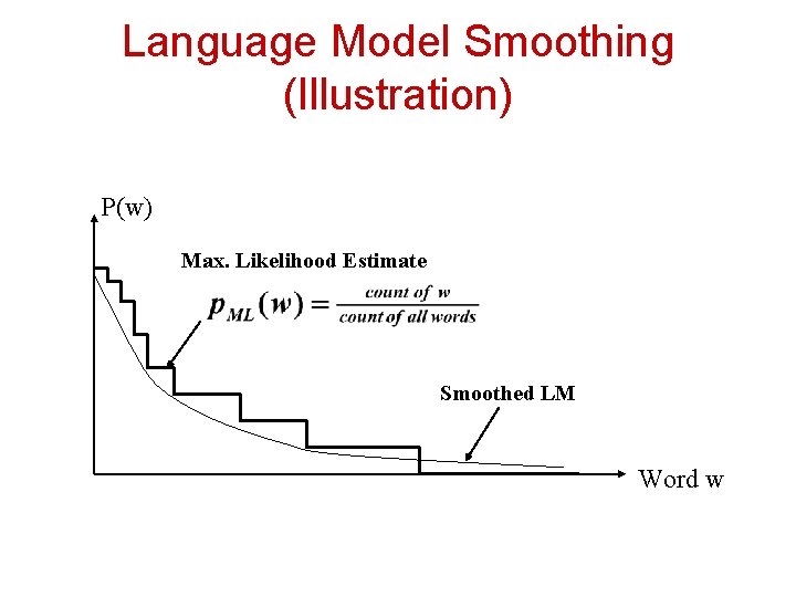
How to Estimate p(w|d)? • Simplest solution: Maximum Likelihood Estimator – P(w|d) = relative frequency of word w in d – What if a word doesn’t appear in the text? P(w|d)=0 • In general, what probability should we give a word that has not been observed? • If we want to assign non-zero probabilities to such words, we’ll have to discount the probabilities of observed words • This is what “smoothing” is about …

Language Model Smoothing (Illustration) P(w) Max. Likelihood Estimate Smoothed LM Word w

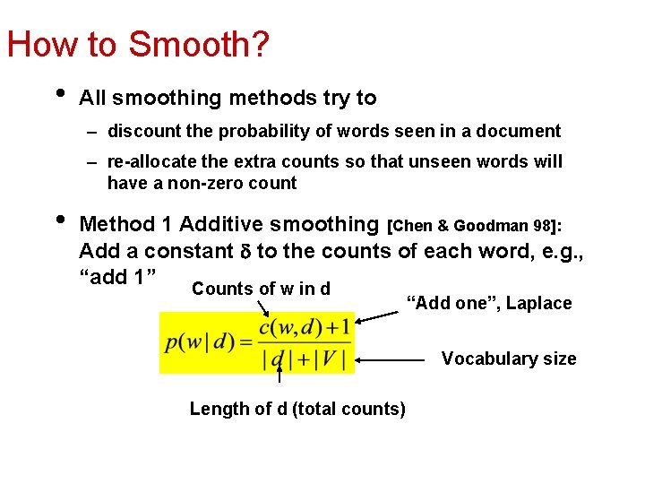
How to Smooth? • All smoothing methods try to – discount the probability of words seen in a document – re-allocate the extra counts so that unseen words will have a non-zero count • Method 1 Additive smoothing [Chen & Goodman 98]: Add a constant to the counts of each word, e. g. , “add 1” Counts of w in d “Add one”, Laplace Vocabulary size Length of d (total counts)

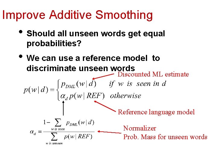
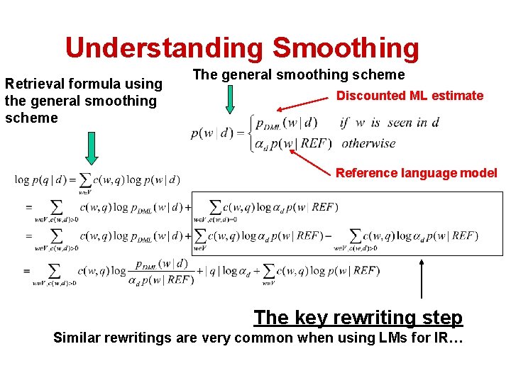
Improve Additive Smoothing • Should all unseen words get equal probabilities? • We can use a reference model to discriminate unseen words Discounted ML estimate Reference language model Normalizer Prob. Mass for unseen words

Other Smoothing Methods • Method 2 Absolute discounting [Ney et al. 94]: Subtract a constant from the counts of each word # unique words • Method 3 Linear interpolation [Jelinek-Mercer 80]: “Shrink” uniformly toward p(w|REF) ML estimate parameter

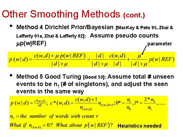
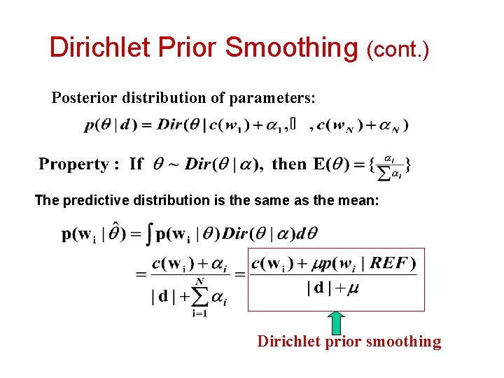
Other Smoothing Methods (cont. ) • • Method 4 Dirichlet Prior/Bayesian [Mac. Kay & Peto 95, Zhai & Lafferty 01 a, Zhai & Lafferty 02]: Assume pseudo counts p(w|REF) parameter Method 5 Good Turing [Good 53]: Assume total # unseen events to be n 1 (# of singletons), and adjust the seen events in the same way Heuristics needed

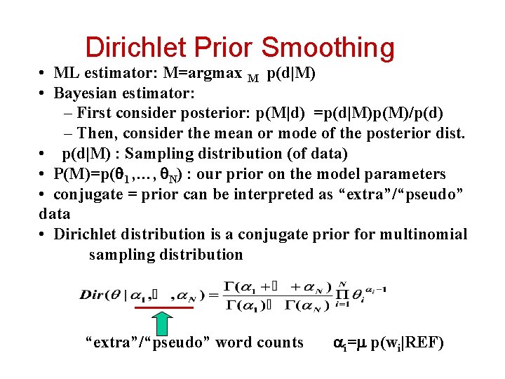
Dirichlet Prior Smoothing • ML estimator: M=argmax M p(d|M) • Bayesian estimator: – First consider posterior: p(M|d) =p(d|M)p(M)/p(d) – Then, consider the mean or mode of the posterior dist. • p(d|M) : Sampling distribution (of data) • P(M)=p( 1 , …, N) : our prior on the model parameters • conjugate = prior can be interpreted as “extra”/“pseudo” data • Dirichlet distribution is a conjugate prior for multinomial sampling distribution “extra”/“pseudo” word counts i= p(wi|REF)

Dirichlet Prior Smoothing (cont. ) Posterior distribution of parameters: The predictive distribution is the same as the mean: Dirichlet prior smoothing

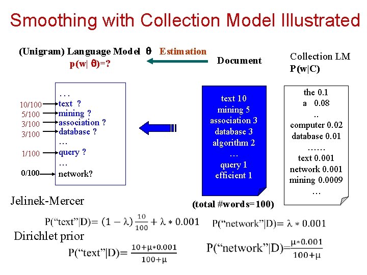
Smoothing with Collection Model Illustrated (Unigram) Language Model Estimation Document p(w| )=? … 10/100 5/100 3/100 1/100 0/100 text ? mining ? association ? database ? … query ? … network? Jelinek-Mercer Dirichlet prior text 10 mining 5 association 3 database 3 algorithm 2 … query 1 efficient 1 (total #words=100) Collection LM P(w|C) the 0. 1 a 0. 08. . computer 0. 02 database 0. 01 …… text 0. 001 network 0. 001 mining 0. 0009 …

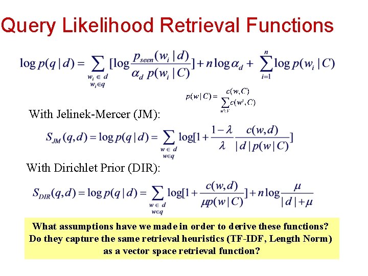
Query Likelihood Retrieval Functions With Jelinek-Mercer (JM): With Dirichlet Prior (DIR): What assumptions have we made in order to derive these functions? Do they capture the same retrieval heuristics (TF-IDF, Length Norm) as a vector space retrieval function?

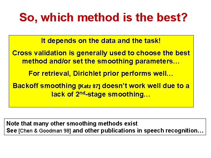
So, which method is the best? It depends on the data and the task! Cross validation is generally used to choose the best method and/or set the smoothing parameters… For retrieval, Dirichlet prior performs well… Backoff smoothing [Katz 87] doesn’t work well due to a lack of 2 nd-stage smoothing… Note that many other smoothing methods exist See [Chen & Goodman 98] and other publications in speech recognition…

Comparison of Three Methods [Zhai & Lafferty 01 a] Comparison is performed on a variety of test collections

Understanding Smoothing Retrieval formula using the general smoothing scheme The general smoothing scheme Discounted ML estimate Reference language model The key rewriting step Similar rewritings are very common when using LMs for IR…

Smoothing & TF-IDF Weighting [Zhai & Lafferty 01 a] • Plug in the general smoothing scheme to the query likelihood retrieval formula, we obtain TF weighting Words in both query and doc • • Doc length normalization (long doc is expected to have a smaller d) IDF-like weighting Ignore for ranking Smoothing with p(w|C) TF-IDF + length norm. Smoothing implements traditional retrieval heuristics LMs with simple smoothing can be computed as efficiently as traditional retrieval models

The Dual-Role of Smoothing [Zhai & Lafferty 02] long Verbose queries Keyword queries long short Why does query type affect smoothing sensitivity?

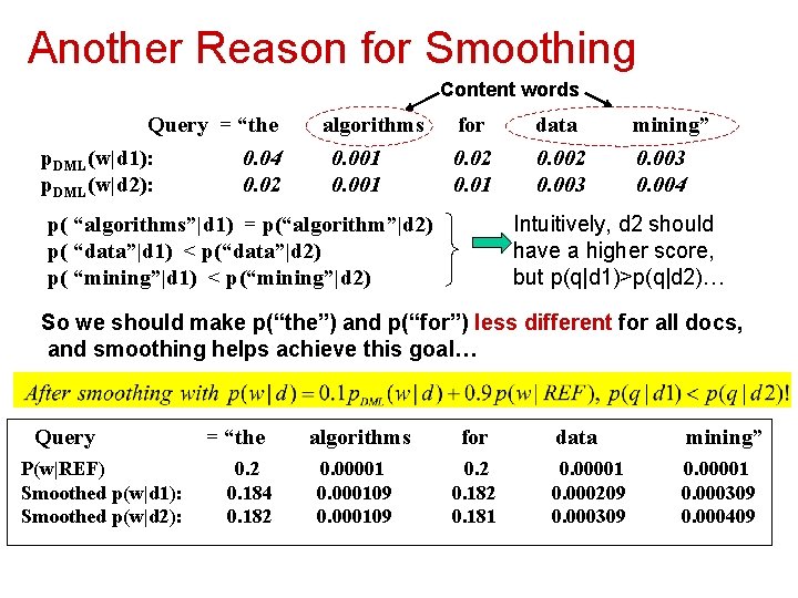
Another Reason for Smoothing Content words Query = “the p. DML(w|d 1): p. DML(w|d 2): 0. 04 0. 02 algorithms 0. 001 for data mining” 0. 02 0. 01 0. 002 0. 003 0. 004 Intuitively, d 2 should have a higher score, but p(q|d 1)>p(q|d 2)… p( “algorithms”|d 1) = p(“algorithm”|d 2) p( “data”|d 1) < p(“data”|d 2) p( “mining”|d 1) < p(“mining”|d 2) So we should make p(“the”) and p(“for”) less different for all docs, and smoothing helps achieve this goal… Query P(w|REF) Smoothed p(w|d 1): Smoothed p(w|d 2): = “the 0. 2 0. 184 0. 182 algorithms for 0. 00001 0. 000109 0. 2 0. 181 data mining” 0. 00001 0. 000209 0. 000309 0. 00001 0. 000309 0. 000409

Two-stage Smoothing [Zhai & Lafferty 02] Stage-2 Stage-1 -Explain noise in query -Explain unseen words -Dirichlet prior(Bayesian) -2 -component mixture P(w|d) = (1 - ) c(w, d) + p(w|C) |d| + Collection LM + p(w|U) User background model Can be approximated by p(w|C)

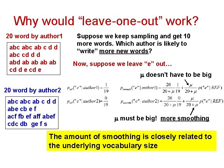
Estimating using leave-one-out [Zhai & Lafferty 02] w 1 P(w 1|d- w 1) log-likelihood Leave-one-out w 2 P(w 2|d- w 2) Maximum Likelihood Estimator . . . wn P(wn|d- wn) Newton’s Method

Why would “leave-one-out” work? 20 word by author 1 abc ab c d d abc cd d d ab ab cd d e cd e Suppose we keep sampling and get 10 more words. Which author is likely to “write” more new words? Now, suppose we leave “e” out… doesn’t have to be big 20 word by author 2 abc ab c d d abe cb e f acf fb ef aff abef cdc db ge f s must be big! more smoothing The amount of smoothing is closely related to the underlying vocabulary size

Estimating using Mixture Model [Zhai & Lafferty 02] Stage-2 Stage-1 d 1 P(w|d 1) (1 - )p(w|d 1)+ p(w|U) . . . …. . . d. N P(w|d. N) 1 N Query Q=q 1…qm (1 - )p(w|d. N)+ p(w|U) Estimated in stage-1 Maximum Likelihood Estimator Expectation-Maximization (EM) algorithm

Automatic 2 -stage results Optimal 1 -stage results [Zhai & Lafferty 02] Average precision (3 DB’s + 4 query types, 150 topics) * Indicates significant difference Completely automatic tuning of parameters IS POSSIBLE!

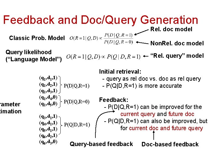
Feedback and Doc/Query Generation Rel. doc model Classic Prob. Model Non. Rel. doc model Query likelihood (“Language Model”) rameter timation (q 1, d 1, 1) (q 1, d 2, 1) (q 1, d 3, 1) (q 1, d 4, 0) (q 1, d 5, 0) (q 3, d 1, 1) (q 4, d 1, 1) (q 5, d 1, 1) (q 6, d 2, 1) (q 6, d 3, 0) “Rel. query” model P(D|Q, R=1) P(D|Q, R=0) P(Q|D, R=1) Initial retrieval: - query as rel doc vs. doc as rel query - P(Q|D, R=1) is more accurate Feedback: - P(D|Q, R=1) can be improved for the current query and future doc - P(Q|D, R=1) can also be improved, but for current doc and future query Query-based feedback Doc-based feedback

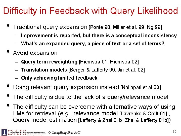
Difficulty in Feedback with Query Likelihood • Traditional query expansion [Ponte 98, Miller et al. 99, Ng 99] – Improvement is reported, but there is a conceptual inconsistency • – What’s an expanded query, a piece of text or a set of terms? Avoid expansion – Query term reweighting [Hiemstra 01, Hiemstra 02] – Translation models [Berger & Lafferty 99, Jin et al. 02] • • • – Only achieving limited feedback Doing relevant query expansion instead [Nallapati et al 03] The difficulty is due to the lack of a query/relevance model The difficulty can be overcome with alternative ways of using LMs for retrieval (e. g. , relevance model [Lavrenko & Croft 01] , Query model estimation [Lafferty & Zhai 01 b; Zhai & Lafferty 01 b]) © Cheng. Xiang Zhai, 2007 30

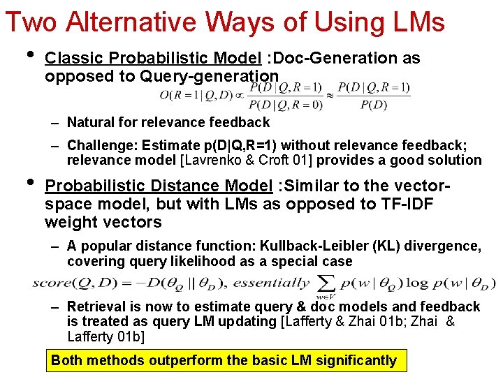
Two Alternative Ways of Using LMs • Classic Probabilistic Model : Doc-Generation as opposed to Query-generation – Natural for relevance feedback • – Challenge: Estimate p(D|Q, R=1) without relevance feedback; relevance model [Lavrenko & Croft 01] provides a good solution Probabilistic Distance Model : Similar to the vectorspace model, but with LMs as opposed to TF-IDF weight vectors – A popular distance function: Kullback-Leibler (KL) divergence, covering query likelihood as a special case – Retrieval is now to estimate query & doc models and feedback is treated as query LM updating [Lafferty & Zhai 01 b; Zhai & Lafferty 01 b] Both methods outperform the basic LM significantly

Query Model Estimation [Lafferty & Zhai 01 b, Zhai & Lafferty 01 b] • • Question: How to estimate a better query model than the ML estimate based on the original query? “Massive feedback”: Improve a query model through co-occurrence pattern learned from – A document-term Markov chain that outputs the query [Lafferty & Zhai 01 b] • – Thesauri, corpus [Bai et al. 05, Collins-Thompson & Callan 05] Model-based feedback: Improve the estimate of query model by exploiting pseudo-relevance feedback – Update the query model by interpolating the original query model with a learned feedback model [ Zhai & Lafferty 01 b] – Estimate a more integrated mixture model using pseudofeedback documents [ Tao & Zhai 06]

Feedback as Model Interpolation [Zhai & Lafferty 01 b] Document D Results Query Q =0 Feedback Docs F={d 1, d 2 , …, dn} =1 Generative model No feedback Full feedback Divergence minimization

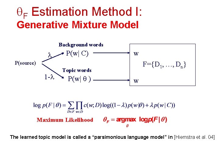
F Estimation Method I: Generative Mixture Model Background words P(w| C) w P(source) 1 - F={D 1, …, Dn} Topic words P(w| ) w Maximum Likelihood The learned topic model is called a “parsimonious language model” in [Hiemstra et al. 04]

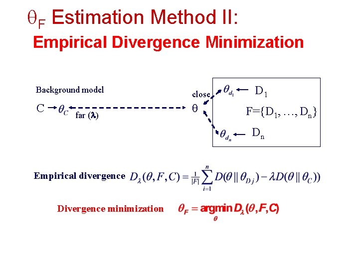
F Estimation Method II: Empirical Divergence Minimization Background model close C far ( ) D 1 F={D 1, …, Dn} Dn Empirical divergence Divergence minimization

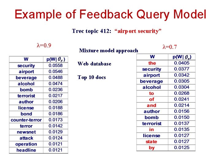
Example of Feedback Query Model Trec topic 412: “airport security” =0. 9 Mixture model approach Web database Top 10 docs =0. 7

Model-based feedback Improves over Simple LM [Zhai & Lafferty 01 b]

What You Should Know • • • Derivation of query likelihood retrieval model using query generation (what are the assumptions made? ) Dirichlet prior and Jelinek Mercer smoothing methods Connection between query likelihood and TF-IDF weighting + doc length normalization The basic idea of two-stage smoothing KL-divergence retrieval model Basic idea of feedback methods (mixture model)