Information Retrieval Models and Methods Roadmap Problem Matching

Information Retrieval: Models and Methods

Roadmap • Problem: – Matching Topics and Documents • Methods: – Classic: Vector Space Model – N-grams – HMMs • Challenge: Beyond literal matching – Expansion Strategies – Aspect Models

Matching Topics and Documents • Two main perspectives: – Pre-defined, fixed, finite topics: • “Text Classification” – Arbitrary topics, typically defined by statement of information need (aka query) • “Information Retrieval”

Matching Topics and Documents • Documents are “about” some topic(s) • Question: Evidence of “aboutness”? – Words !! • Possibly also meta-data in documents – Tags, etc • Model encodes how words capture topic – E. g. “Bag of words” model, Boolean matching – What information is captured? – How is similarity computed?

Models for Retrieval and Classification • Plethora of models are used • Here: – Vector Space Model – N-grams – HMMs

Vector Space Information Retrieval • Task: – Document collection – Query specifies information need: free text – Relevance judgments: 0/1 for all docs • Word evidence: Bag of words – No ordering information

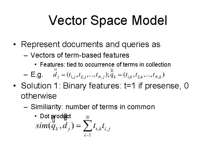
Vector Space Model • Represent documents and queries as – Vectors of term-based features • Features: tied to occurrence of terms in collection – E. g. • Solution 1: Binary features: t=1 if presense, 0 otherwise – Similiarity: number of terms in common • Dot product

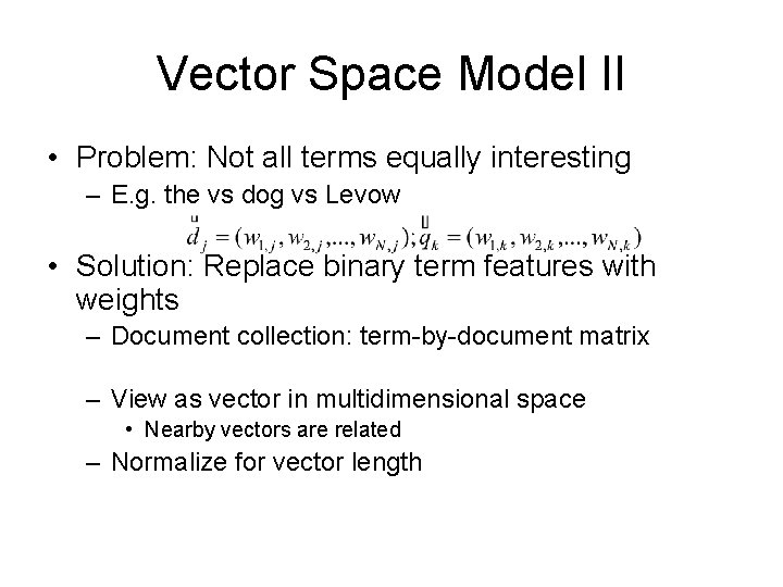
Vector Space Model II • Problem: Not all terms equally interesting – E. g. the vs dog vs Levow • Solution: Replace binary term features with weights – Document collection: term-by-document matrix – View as vector in multidimensional space • Nearby vectors are related – Normalize for vector length

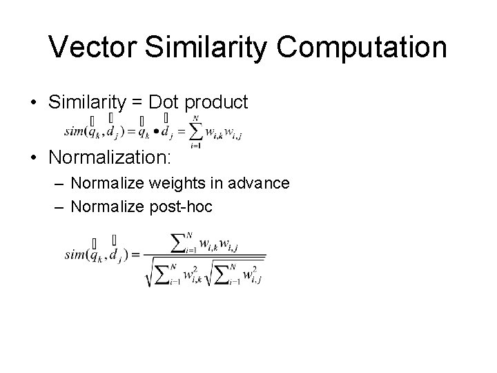
Vector Similarity Computation • Similarity = Dot product • Normalization: – Normalize weights in advance – Normalize post-hoc

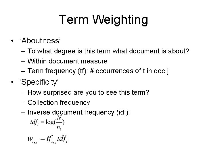
Term Weighting • “Aboutness” – To what degree is this term what document is about? – Within document measure – Term frequency (tf): # occurrences of t in doc j • “Specificity” – How surprised are you to see this term? – Collection frequency – Inverse document frequency (idf):

Term Selection & Formation • Selection: – Some terms are truly useless • Too frequent, no content – E. g. the, a, and, … – Stop words: ignore such terms altogether • Creation: – Too many surface forms for same concepts • E. g. inflections of words: verb conjugations, plural – Stem terms: treat all forms as same underlying

N-grams • Simple model • Evidence: More than bag of words – Captures context, order information • E. g. White House • Applicable to many text tasks – Language identification, authorship attribution, genre classification, topic/text classification – Language modeling for ASR, etc

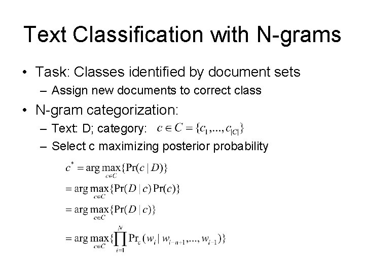
Text Classification with N-grams • Task: Classes identified by document sets – Assign new documents to correct class • N-gram categorization: – Text: D; category: – Select c maximizing posterior probability

Text Classification with N-grams • Representation: – For each class, train N-gram model • “Similarity”: For each document D to classify, select c with highest likelihood – Can also use entropy/perplexity

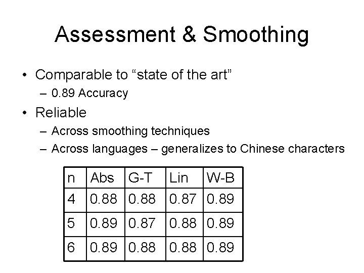
Assessment & Smoothing • Comparable to “state of the art” – 0. 89 Accuracy • Reliable – Across smoothing techniques – Across languages – generalizes to Chinese characters n 4 Abs G-T Lin W-B 0. 88 0. 87 0. 89 5 0. 89 0. 87 0. 88 0. 89 6 0. 89 0. 88 0. 89

HMMs • Provides a generative model of topicality – Solid probabilistic framework rather than ad hoc weighting • Noisy channel model: – View query Q as output of underlying relevant document D, passed through mind of user

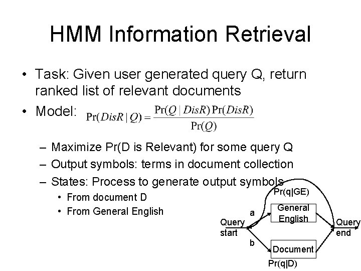
HMM Information Retrieval • Task: Given user generated query Q, return ranked list of relevant documents • Model: – Maximize Pr(D is Relevant) for some query Q – Output symbols: terms in document collection – States: Process to generate output symbols • From document D • From General English Pr(q|GE) Query start a b General English Document Pr(q|D) Query end

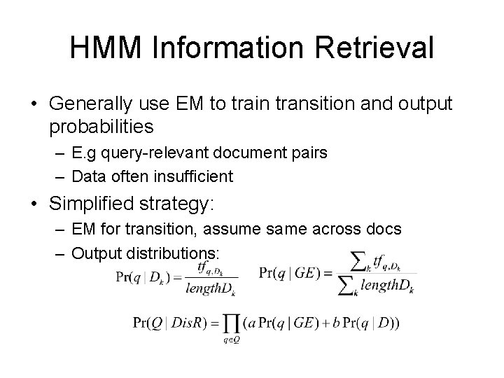
HMM Information Retrieval • Generally use EM to train transition and output probabilities – E. g query-relevant document pairs – Data often insufficient • Simplified strategy: – EM for transition, assume same across docs – Output distributions:

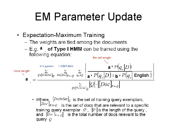
EM Parameter Update a a‘ b‘ English

Evaluation • Comparison to VSM – HMM can outperform VSM • Some variation related to implementation – Can integrate other features –e. g. bigram or trigram models,

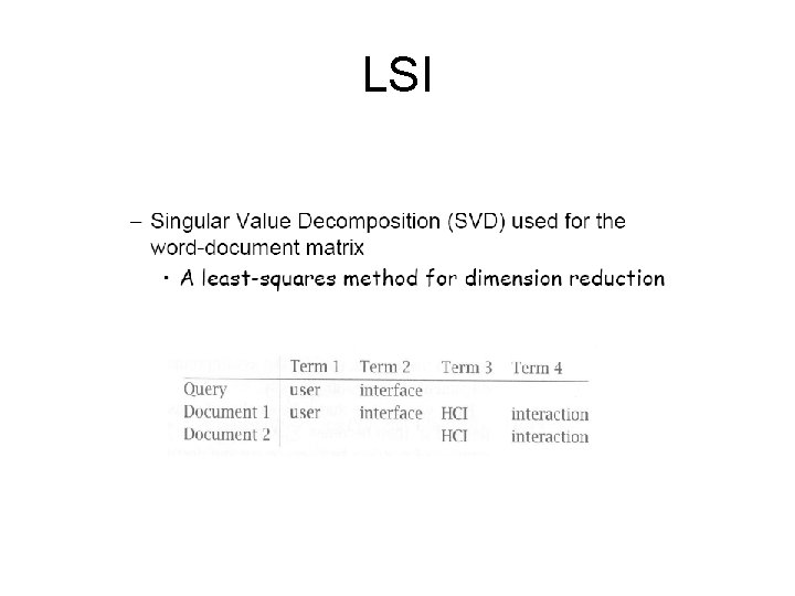
Key Issue • All approaches operate on term matching – If a synonym, rather than original term, is used, approach fails • Develop more robust techniques – Match “concept” rather than term • Expansion approaches – Add in related terms to enhance matching • Mapping techniques – Associate terms to concepts » Aspect models, stemming

Expansion Techniques • Can apply to query or document • Thesaurus expansion – Use linguistic resource – thesaurus, Word. Net – to add synonyms/related terms • Feedback expansion – Add terms that “should have appeared” • User interaction – Direct or relevance feedback • Automatic pseudo relevance feedback

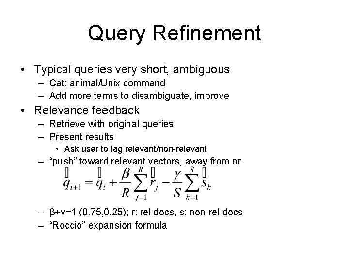
Query Refinement • Typical queries very short, ambiguous – Cat: animal/Unix command – Add more terms to disambiguate, improve • Relevance feedback – Retrieve with original queries – Present results • Ask user to tag relevant/non-relevant – “push” toward relevant vectors, away from nr – β+γ=1 (0. 75, 0. 25); r: rel docs, s: non-rel docs – “Roccio” expansion formula

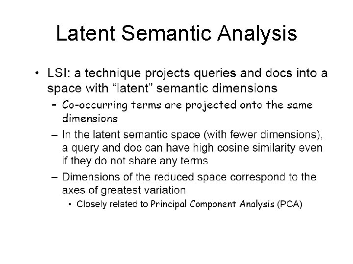
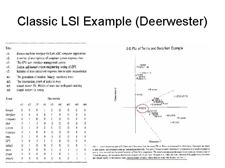
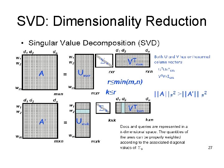
Compression Techniques • Reduce surface term variation to concepts • Stemming – Map inflectional variants to root • E. g. see, sees, seen, saw -> see • Crucial for highly inflected languages – Czech, Arabic • Aspect models – Matrix representations typically very sparse – Reduce dimensionality to small # key aspects • Mapping contextually similar terms together • Latent semantic analysis

Latent Semantic Analysis

Latent Semantic Analysis

LSI

Classic LSI Example (Deerwester)

SVD: Dimensionality Reduction

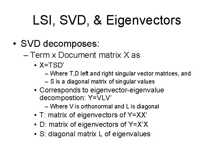
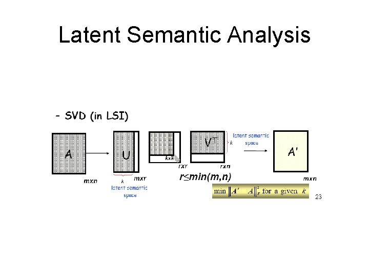
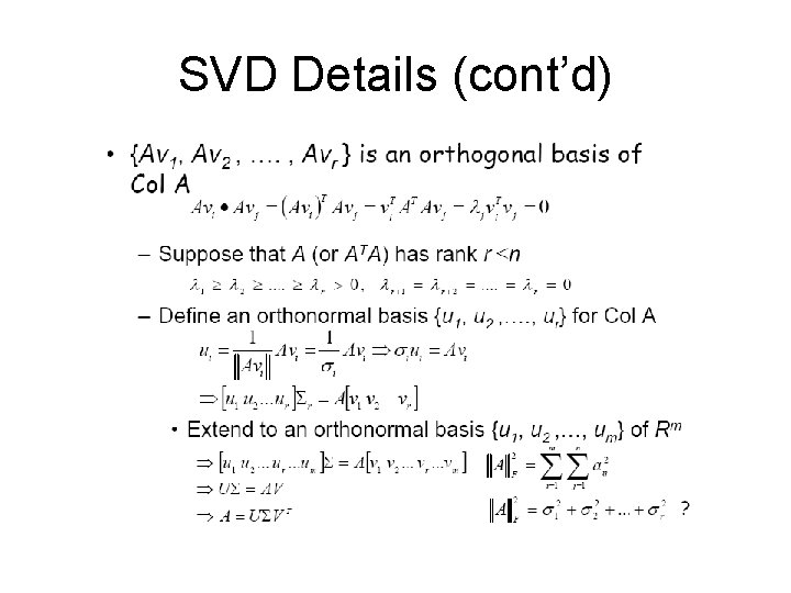
LSI, SVD, & Eigenvectors • SVD decomposes: – Term x Document matrix X as • X=TSD’ – Where T, D left and right singular vector matrices, and – S is a diagonal matrix of singular values • Corresponds to eigenvector-eigenvalue decompostion: Y=VLV’ – Where V is orthonormal and L is diagonal • T: matrix of eigenvectors of Y=XX’ • D: matrix of eigenvectors of Y=X’X • S: diagonal matrix L of eigenvalues

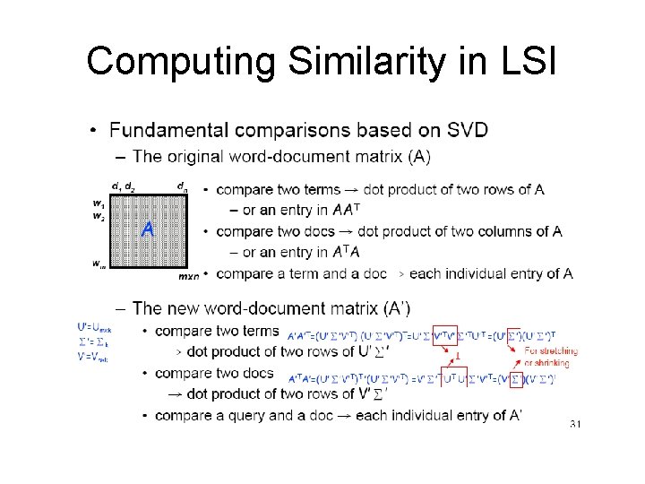
Computing Similarity in LSI

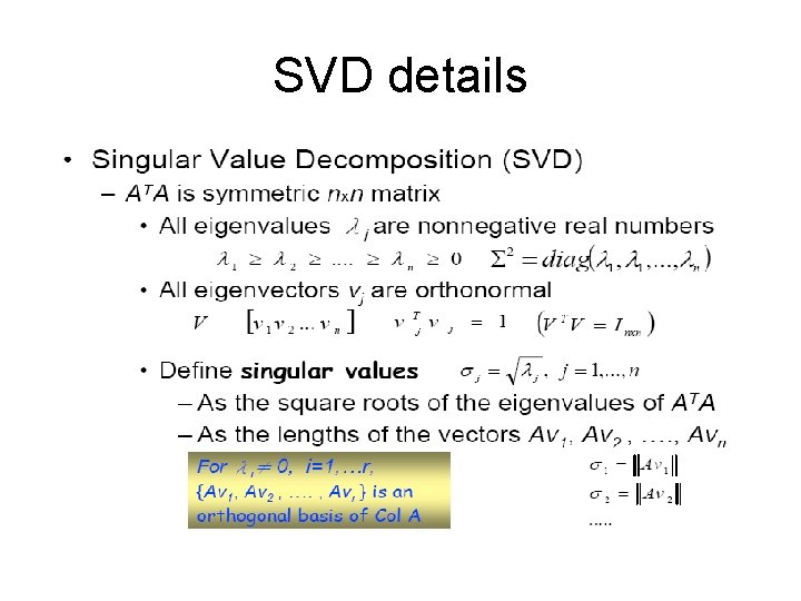
SVD details

SVD Details (cont’d)