Information Retrieval Data compression Architectural features CPU L

Information Retrieval Data compression

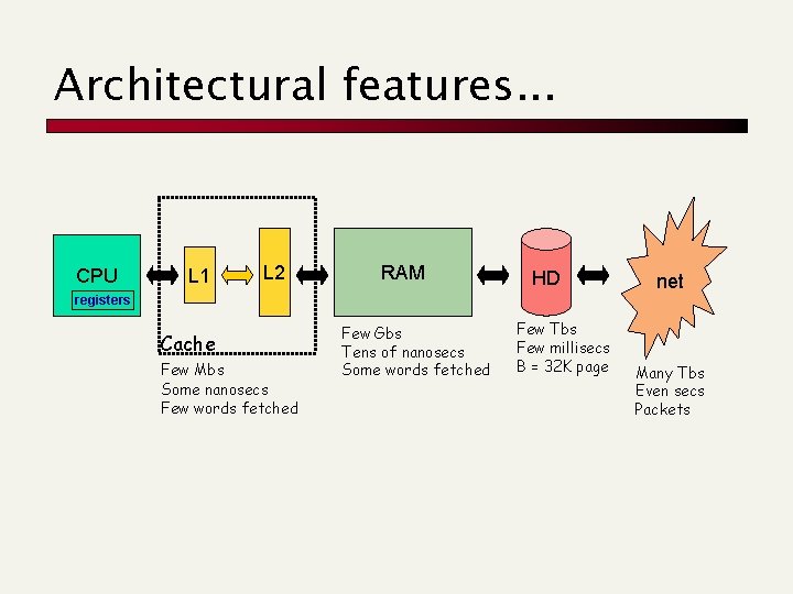
Architectural features. . . CPU L 1 L 2 RAM HD net registers Cache Few Mbs Some nanosecs Few words fetched Few Gbs Tens of nanosecs Some words fetched Few Tbs Few millisecs B = 32 K page Many Tbs Even secs Packets

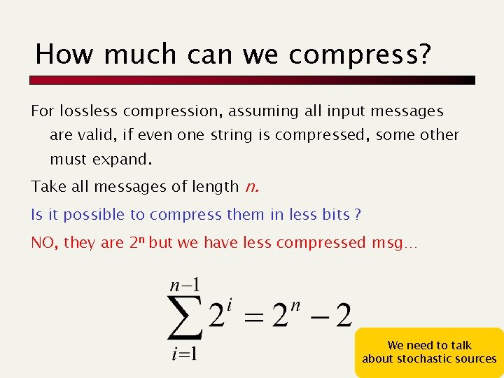
How much can we compress? For lossless compression, assuming all input messages are valid, if even one string is compressed, some other must expand. Take all messages of length n. Is it possible to compress them in less bits ? NO, they are 2 n but we have less compressed msg… We need to talk about stochastic sources

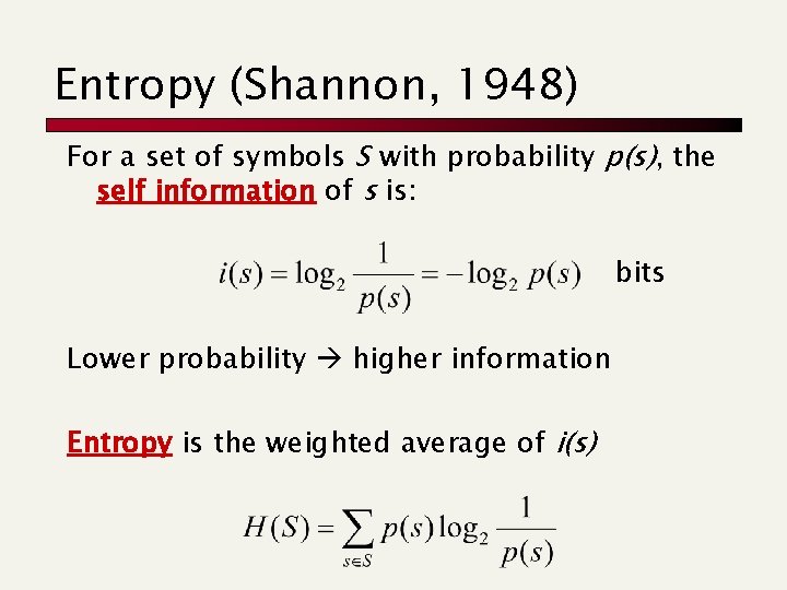
Entropy (Shannon, 1948) For a set of symbols S with probability p(s), the self information of s is: bits Lower probability higher information Entropy is the weighted average of i(s)

Statistical Coding How do we use the p(s) to encode s? n n n Prefix codes and relationship to Entropy Huffman codes Arithmetic codes

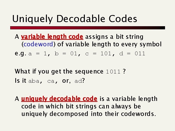
Uniquely Decodable Codes A variable length code assigns a bit string (codeword) of variable length to every symbol e. g. a = 1, b = 01, c = 101, d = 011 What if you get the sequence 1011 ? Is it aba, ca, or, ad? A uniquely decodable code is a variable length code in which bit strings can always be uniquely decomposed into their codewords.

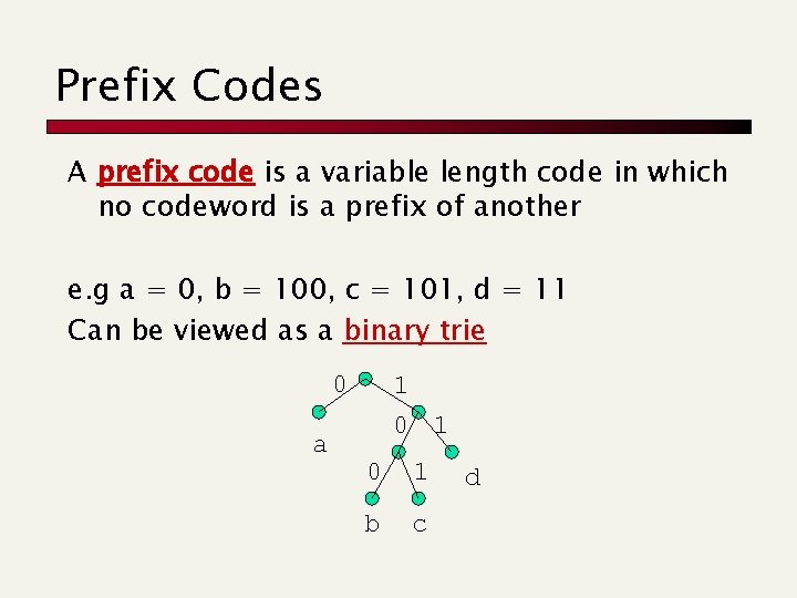
Prefix Codes A prefix code is a variable length code in which no codeword is a prefix of another e. g a = 0, b = 100, c = 101, d = 11 Can be viewed as a binary trie 0 a 1 0 1 b c d

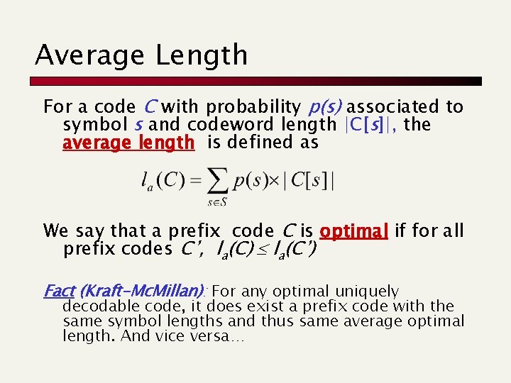
Average Length For a code C with probability p(s) associated to symbol s and codeword length |C[s]|, the average length is defined as We say that a prefix code C is optimal if for all prefix codes C’, la(C) la(C’) Fact (Kraft-Mc. Millan): For any optimal uniquely decodable code, it does exist a prefix code with the same symbol lengths and thus same average optimal length. And vice versa…

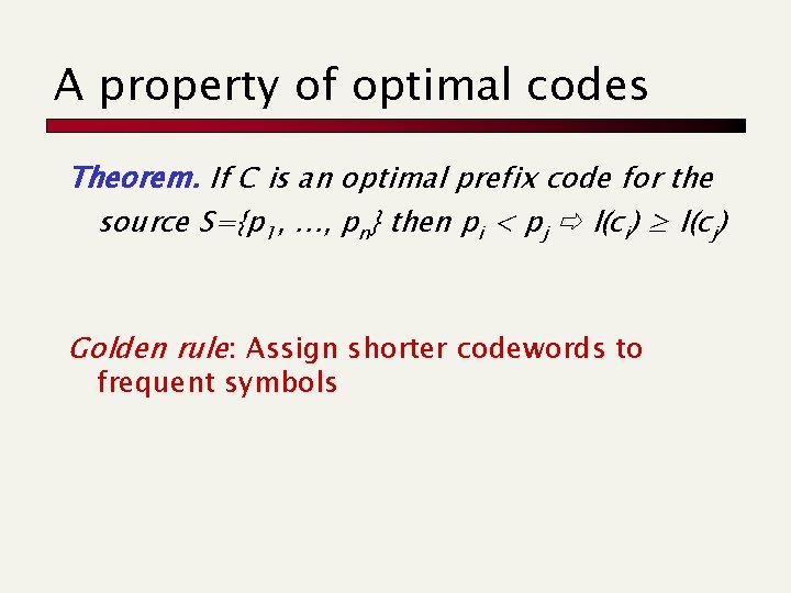
A property of optimal codes Theorem. If C is an optimal prefix code for the source S={p 1, …, pn} then pi < pj l(ci) ≥ l(cj) Golden rule: Assign shorter codewords to frequent symbols

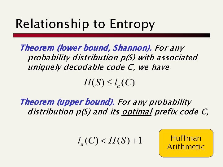
Relationship to Entropy Theorem (lower bound, Shannon). For any probability distribution p(S) with associated uniquely decodable code C, we have Theorem (upper bound). For any probability distribution p(S) and its optimal prefix code C, Huffman Arithmetic

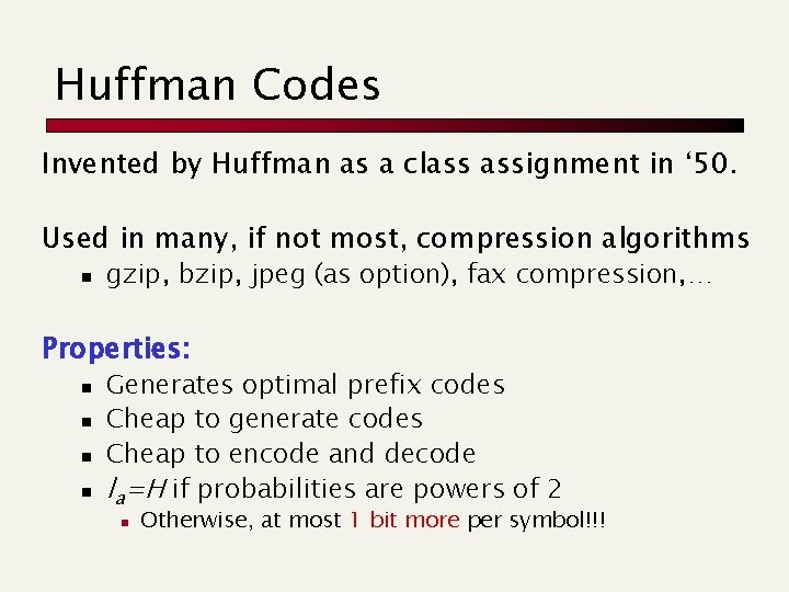
Huffman Codes Invented by Huffman as a class assignment in ‘ 50. Used in many, if not most, compression algorithms n gzip, bzip, jpeg (as option), fax compression, … Properties: n n Generates optimal prefix codes Cheap to generate codes Cheap to encode and decode la=H if probabilities are powers of 2 n Otherwise, at most 1 bit more per symbol!!!

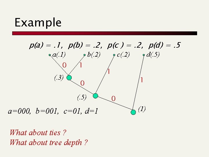
Example p(a) =. 1, p(b) =. 2, p(c ) =. 2, p(d) =. 5 a(. 1) 0 (. 3) b(. 2) 1 c(. 2) 1 1 0 (. 5) a=000, b=001, c=01, d=1 What about ties ? What about tree depth ? d(. 5) 0 (1)

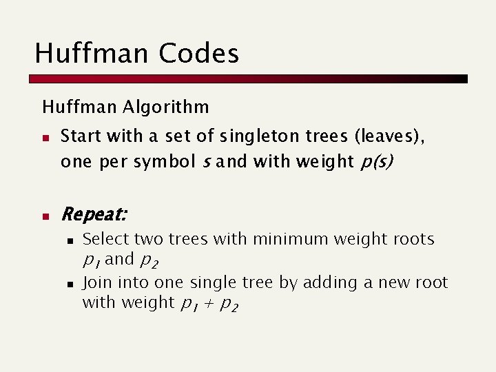
Huffman Codes Huffman Algorithm n n Start with a set of singleton trees (leaves), one per symbol s and with weight p(s) Repeat: n n Select two trees with minimum weight roots p 1 and p 2 Join into one single tree by adding a new root with weight p 1 + p 2

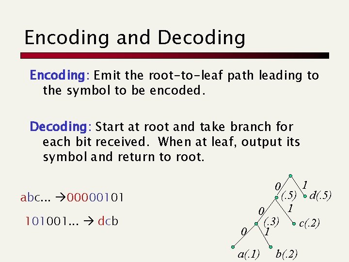
Encoding and Decoding Encoding: Emit the root-to-leaf path leading to the symbol to be encoded. Decoding: Start at root and take branch for each bit received. When at leaf, output its symbol and return to root. 0 abc. . . 00000101 101001. . . dcb 0 0 (. 3) 1 a(. 1) (. 5) 1 b(. 2) 1 d(. 5) c(. 2)

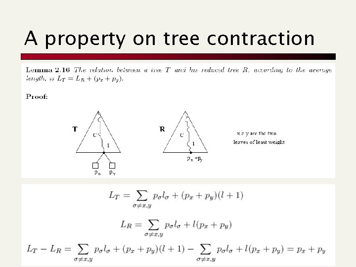
A property on tree contraction

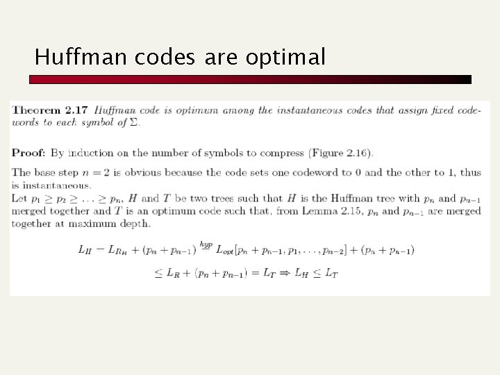
Huffman codes are optimal

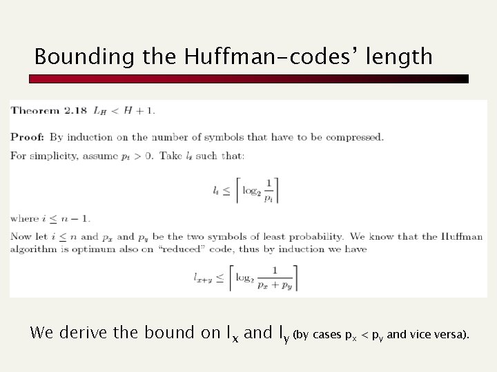
Bounding the Huffman-codes’ length We derive the bound on lx and ly (by cases px < py and vice versa).

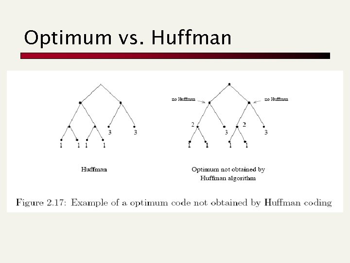
Optimum vs. Huffman

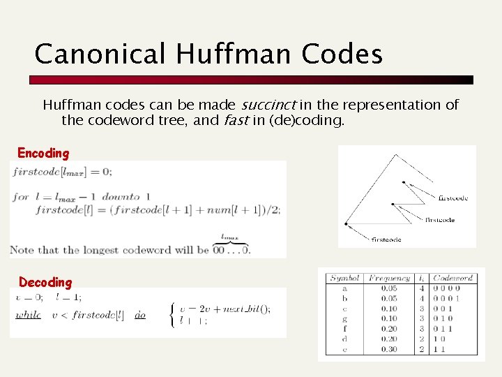
Canonical Huffman Codes Huffman codes can be made succinct in the representation of the codeword tree, and fast in (de)coding. Encoding Decoding

You find this at

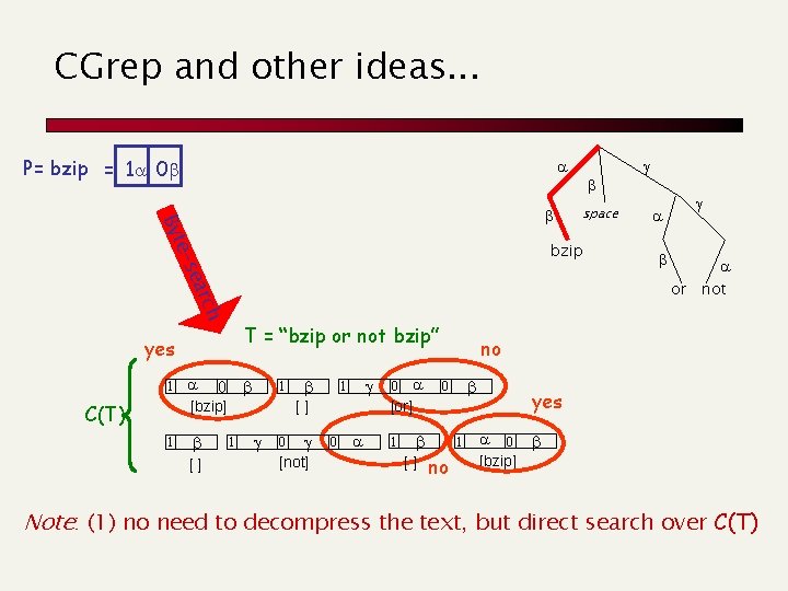
Byte-aligned Huffword [Moura et al, 98] Compressed text derived from a word-based Huffman: ü Symbols of the huffman tree are the words of T ü The Huffman tree has fan-out 128 ü Codewords are byte-aligned and tagged huffman “or” tagging 7 bits a 1 Codeword C(T) 1 a 0 [bzip] [] 1 1 1 [] 0 [not] a 0 a 0 [or] 0 a 1 0 Byte-aligned codeword T = “bzip or not bzip” 1 a 0 space bzip [] 1 a 0 [bzip] a or a not

CGrep and other ideas. . . P= bzip = 1 a 0 a Byt ear e-s 1 T = “bzip or not bzip” a 0 [bzip] [] a or ch C(T) space bzip yes 1 1 [] 0 [not] a 0 no 0 [or] 0 a 1 [] a not 1 no yes a 0 [bzip] Note: (1) no need to decompress the text, but direct search over C(T)

You find this at You find it under my Software projects

Problem with Huffman Coding Consider a message with probability. 999. The self information of this message is If we were to send 1000 such messages we might hope to use 1000*. 0014 = 1. 44 bits. Using Huffman, we take at least one bit per message, so we would require 1000 bits.

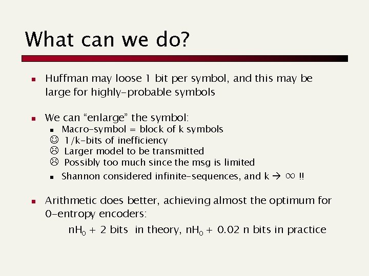
What can we do? n n Huffman may loose 1 bit per symbol, and this may be large for highly-probable symbols We can “enlarge” the symbol: Macro-symbol = block of k symbols J 1/k-bits of inefficiency L Larger model to be transmitted L Possibly too much since the msg is limited n n n Shannon considered infinite-sequences, and k ∞ !! Arithmetic does better, achieving almost the optimum for 0 -entropy encoders: n. H 0 + 2 bits in theory, n. H 0 + 0. 02 n bits in practice

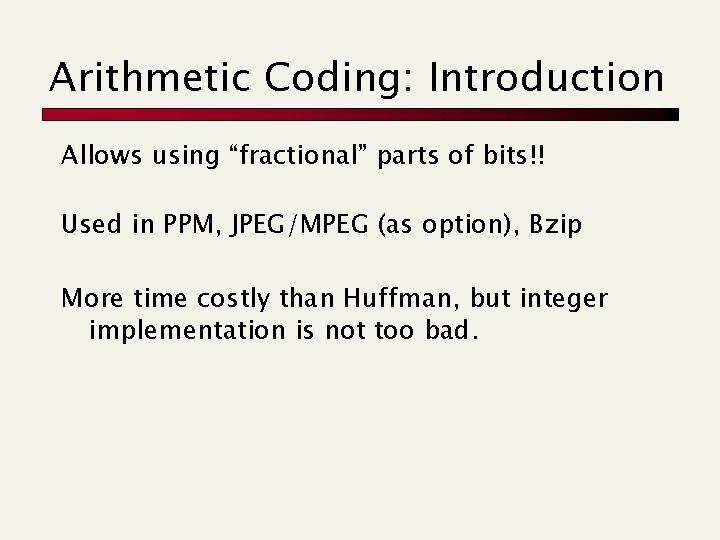
Arithmetic Coding: Introduction Allows using “fractional” parts of bits!! Used in PPM, JPEG/MPEG (as option), Bzip More time costly than Huffman, but integer implementation is not too bad.

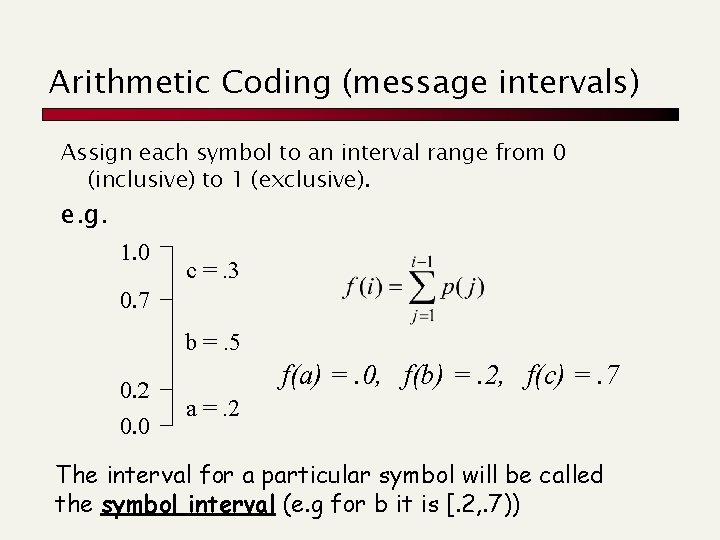
Arithmetic Coding (message intervals) Assign each symbol to an interval range from 0 (inclusive) to 1 (exclusive). e. g. 1. 0 c =. 3 0. 7 b =. 5 0. 2 0. 0 f(a) =. 0, f(b) =. 2, f(c) =. 7 a =. 2 The interval for a particular symbol will be called the symbol interval (e. g for b it is [. 2, . 7))

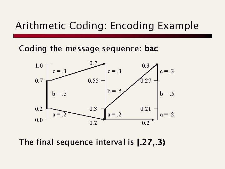
Arithmetic Coding: Encoding Example Coding the message sequence: bac 1. 0 0. 7 c =. 3 0. 55 0. 0 a =. 2 0. 3 0. 2 c =. 3 0. 27 b =. 5 0. 2 0. 3 a =. 2 b =. 5 0. 21 a =. 2 0. 2 The final sequence interval is [. 27, . 3)

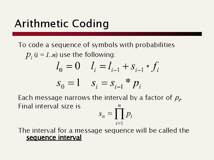
Arithmetic Coding To code a sequence of symbols with probabilities pi (i = 1. . n) use the following: Each message narrows the interval by a factor of pi. Final interval size is The interval for a message sequence will be called the sequence interval

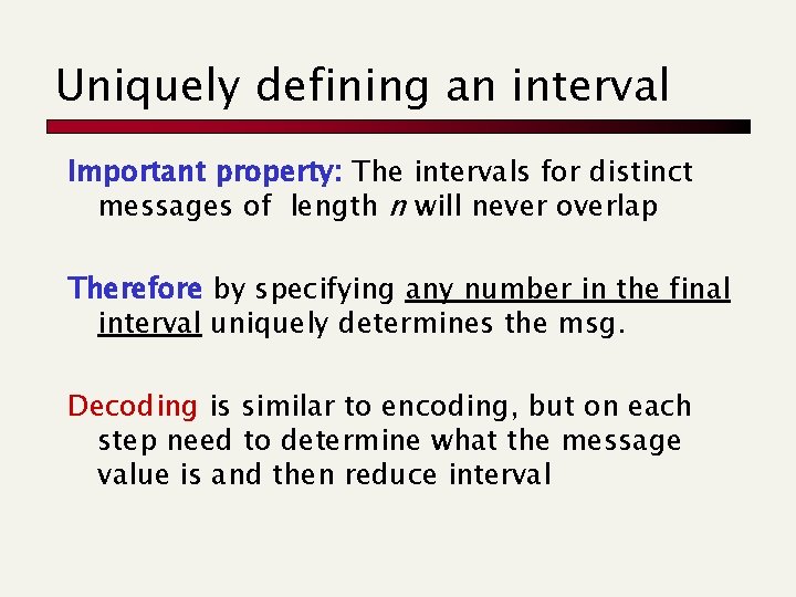
Uniquely defining an interval Important property: The intervals for distinct messages of length n will never overlap Therefore by specifying any number in the final interval uniquely determines the msg. Decoding is similar to encoding, but on each step need to determine what the message value is and then reduce interval

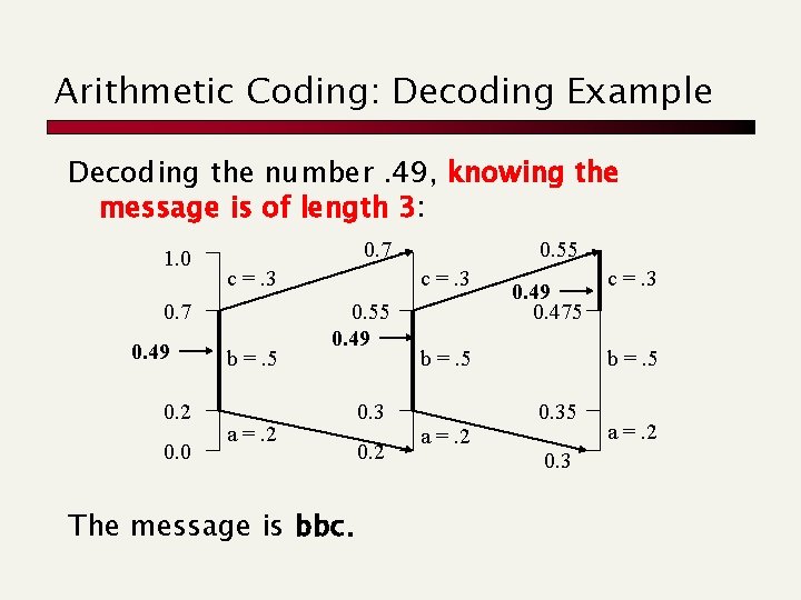
Arithmetic Coding: Decoding Example Decoding the number. 49, knowing the message is of length 3: 1. 0 0. 7 c =. 3 0. 7 0. 49 0. 2 0. 0 b =. 5 0. 55 c =. 3 0. 55 0. 49 a =. 2 The message is bbc. 0. 3 0. 2 0. 49 0. 475 b =. 5 a =. 2 c =. 3 b =. 5 0. 3 a =. 2

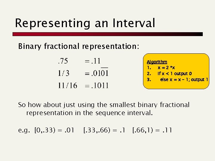
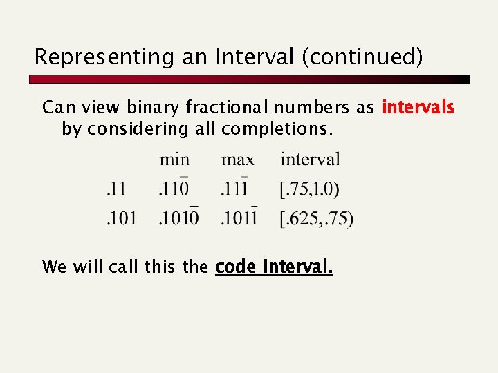
Representing an Interval Binary fractional representation: Algorithm 1. x = 2 *x 2. If x < 1 output 0 3. else x = x - 1; output 1 So how about just using the smallest binary fractional representation in the sequence interval. e. g. [0, . 33) =. 01 [. 33, . 66) =. 1 [. 66, 1) =. 11

Representing an Interval (continued) Can view binary fractional numbers as intervals by considering all completions. We will call this the code interval.

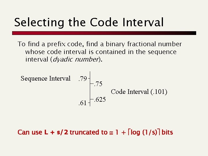
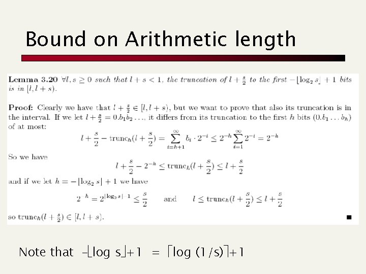
Selecting the Code Interval To find a prefix code, find a binary fractional number whose code interval is contained in the sequence interval (dyadic number). Sequence Interval . 79 . 75 Code Interval (. 101) . 61 . 625 Can use L + s/2 truncated to 1 + log (1/s) bits

Bound on Arithmetic length Note that – log s +1 = log (1/s) +1

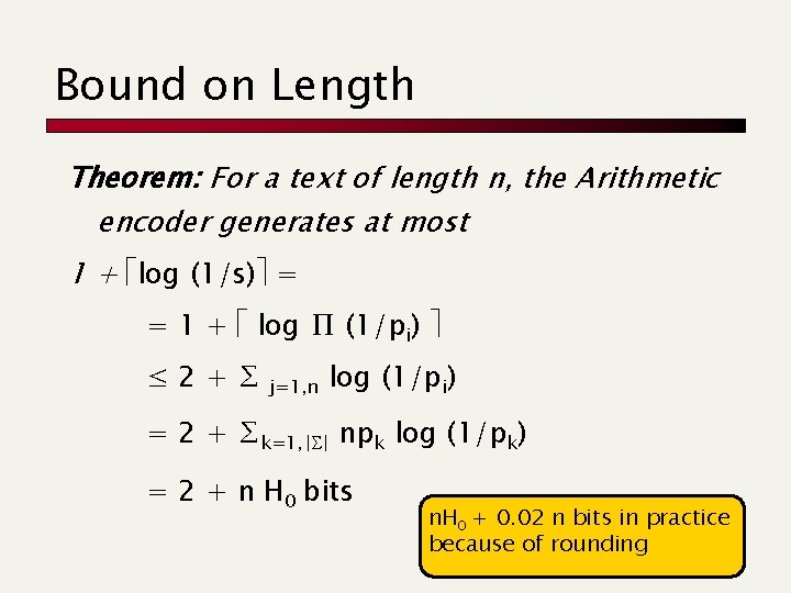
Bound on Length Theorem: For a text of length n, the Arithmetic encoder generates at most 1 + log (1/s) = = 1 + log ∏ (1/pi) ≤ 2+∑ j=1, n log (1/pi) = 2 + ∑k=1, | | npk log (1/pk) = 2 + n H 0 bits n. H 0 + 0. 02 n bits in practice because of rounding

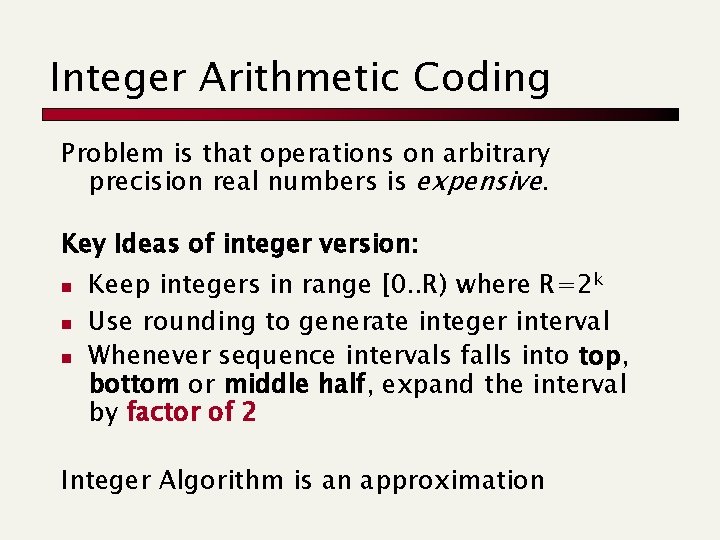
Integer Arithmetic Coding Problem is that operations on arbitrary precision real numbers is expensive. Key Ideas of integer version: n n n Keep integers in range [0. . R) where R=2 k Use rounding to generate integer interval Whenever sequence intervals falls into top, bottom or middle half, expand the interval by factor of 2 Integer Algorithm is an approximation

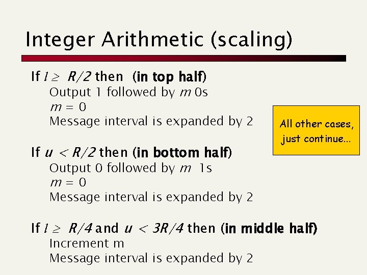
Integer Arithmetic (scaling) If l R/2 then (in top half) Output 1 followed by m 0 s m=0 Message interval is expanded by 2 If u < R/2 then (in bottom half) Output 0 followed by m 1 s m=0 All other cases, just continue. . . Message interval is expanded by 2 If l R/4 and u < 3 R/4 then (in middle half) Increment m Message interval is expanded by 2

You find this at

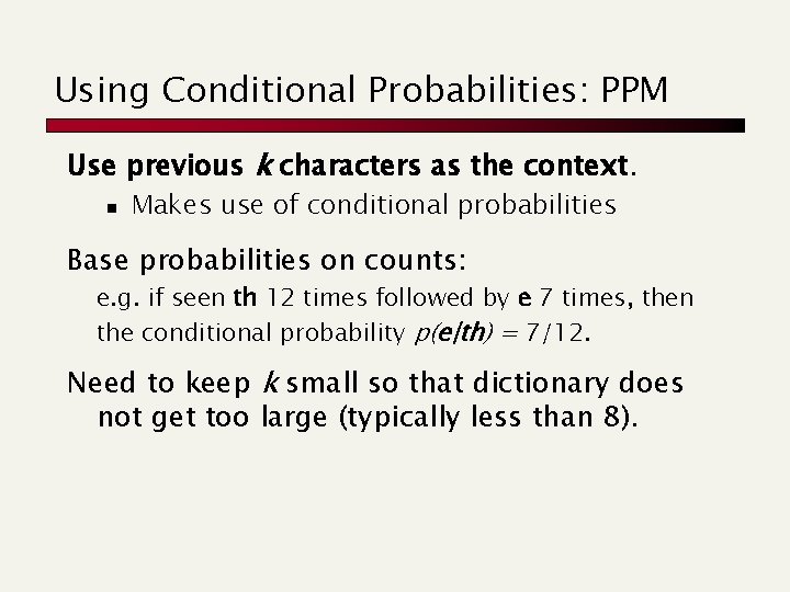
Using Conditional Probabilities: PPM Use previous k characters as the context. n Makes use of conditional probabilities Base probabilities on counts: e. g. if seen th 12 times followed by e 7 times, then the conditional probability p(e|th) = 7/12. Need to keep k small so that dictionary does not get too large (typically less than 8).

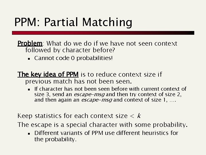
PPM: Partial Matching Problem: What do we do if we have not seen context followed by character before? n Cannot code 0 probabilities! The key idea of PPM is to reduce context size if previous match has not been seen. n If character has not been seen before with current context of size 3, send an escape-msg and then try context of size 2, and then again an escape-msg and context of size 1, …. Keep statistics for each context size < k The escape is a special character with some probability. n Different variants of PPM use different heuristics for the probability.

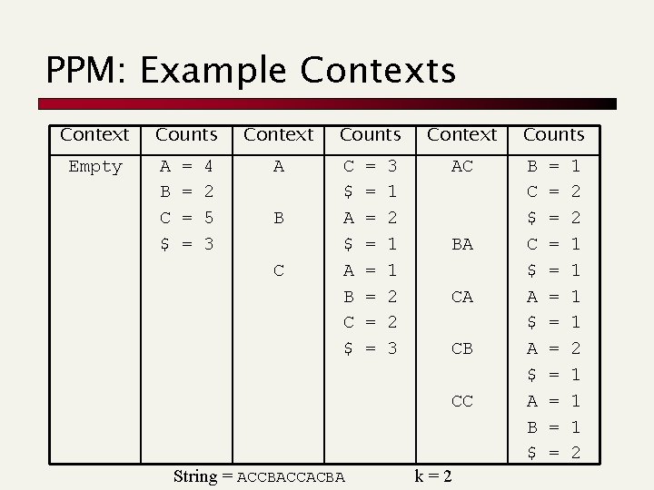
PPM: Example Contexts Context Empty Counts A B C $ = = 4 2 5 3 Context A B C Counts C $ A B C $ = = = = 3 1 2 1 1 2 2 3 Context AC BA CA CB CC String = ACCBACCACBA k=2 Counts B C $ A $ A B $ = = = 1 2 2 1 1 1 2

You find this at: compression. ru/ds/

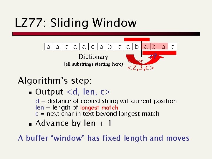
Lempel-Ziv Algorithms Keep a “dictionary” of recently-seen strings. The differences are: n How the dictionary is stored n How it is extended n How it is indexed n How elements are removed No explicit frequency estimation LZ-algos are asymptotically optimal, i. e. their compression ratio goes to H(S) for n !!

LZ 77: Sliding Window a a c a b a c ? ? ? Dictionary Cursor (all substrings starting here) <2, 3, c> Algorithm’s step: n Output <d, len, c> d = distance of copied string wrt current position len = length of longest match c = next char in text beyond longest match n Advance by len + 1 A buffer “window” has fixed length and moves

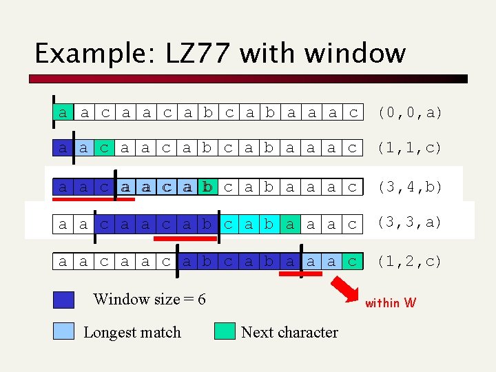
Example: LZ 77 with window a a c a b a a a c (0, 0, a) a a c a b a a a c (1, 1, c) a a c a b a a a c (3, 4, b) a a c a b a a a c (3, 3, a) a a c a b a a a c (1, 2, c) Window size = 6 Longest match within W Next character

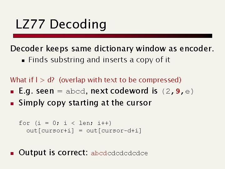
LZ 77 Decoding Decoder keeps same dictionary window as encoder. n Finds substring and inserts a copy of it What if l > d? (overlap with text to be compressed) n n E. g. seen = abcd, next codeword is (2, 9, e) Simply copy starting at the cursor for (i = 0; i < len; i++) out[cursor+i] = out[cursor-d+i] n Output is correct: abcdcdcdce

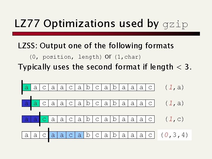
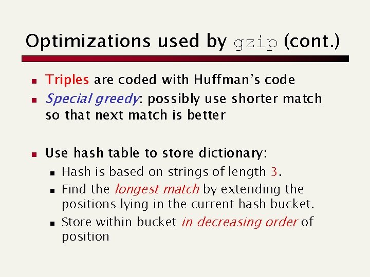
LZ 77 Optimizations used by gzip LZSS: Output one of the following formats (0, position, length) or (1, char) Typically uses the second format if length < 3. a a c a b c a b a a a c (1, a) a a c a b a a a c (1, c) a a c a b a a a c (0, 3, 4)

Optimizations used by gzip (cont. ) n Triples are coded with Huffman’s code Special greedy: possibly use shorter match so that next match is better n Use hash table to store dictionary: n n Hash is based on strings of length 3. Find the longest match by extending the positions lying in the current hash bucket. Store within bucket in decreasing order of position

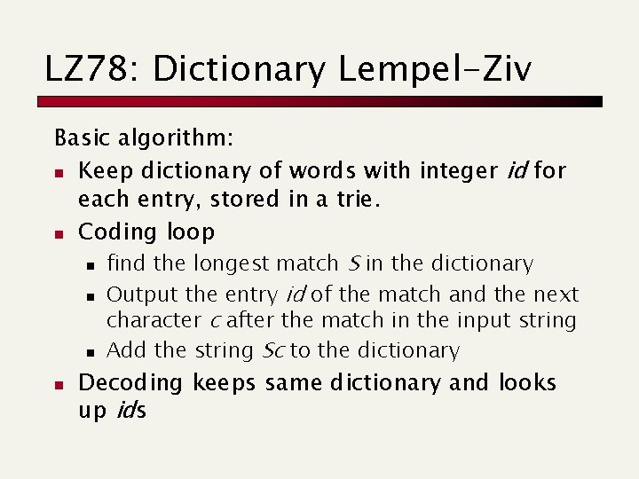
LZ 78: Dictionary Lempel-Ziv Basic algorithm: n Keep dictionary of words with integer id for each entry, stored in a trie. n Coding loop n find the longest match S in the dictionary n Output the entry id of the match and the next character c after the match in the input string n Add the string Sc to the dictionary n Decoding keeps same dictionary and looks up ids

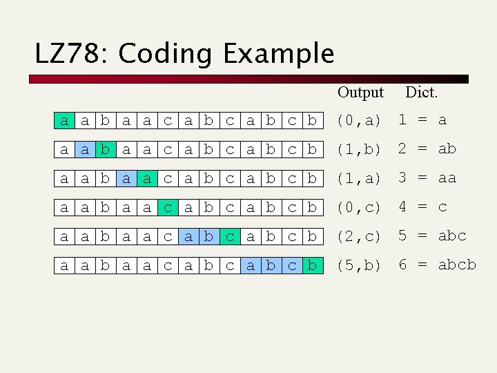
LZ 78: Coding Example Output Dict. a a b a a c a b c b (0, a) 1 = a a a b a a c a b c b (1, b) 2 = ab a a c a b c b (1, a) 3 = aa a a b a a c a b c b (0, c) 4 = c a a b a a c a b c b (2, c) 5 = abc a a b a a c a b c b (5, b) 6 = abcb

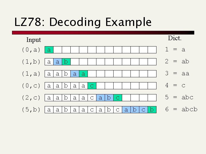
LZ 78: Decoding Example Dict. Input (0, a) a 1 = a (1, b) a a b 2 = ab (1, a) a a b a a 3 = aa (0, c) a a b a a c 4 = c (2, c) a a b a a c a b c 5 = abc (5, b) a a b a a c a b c b 6 = abcb

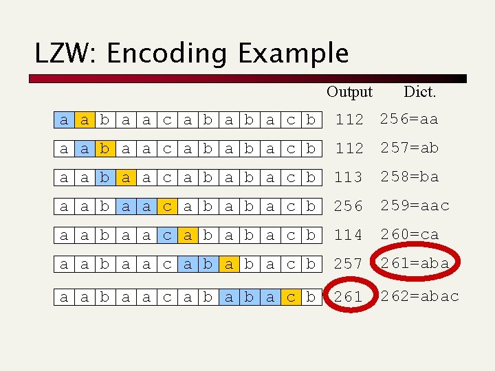
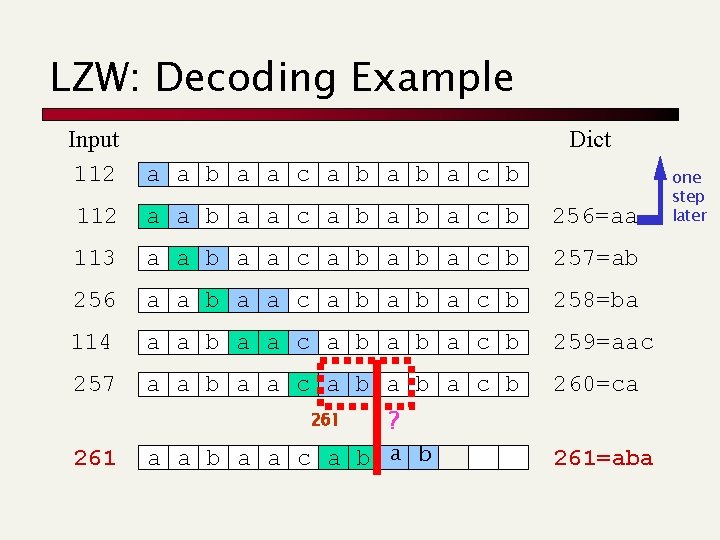
LZW (Lempel-Ziv-Welch) [‘ 84] Don’t send extra character c, but still add Sc to the dictionary. The dictionary is initialized with byte values being the first 256 entries (e. g. a = 112, ascii), otherwise there is no way to start it up. The decoder is one step behind the coder since it does not know c n There is an issue for strings of the form SSc where S[0] = c, and these are handled specially!!!

LZW: Encoding Example Output Dict. a a b a a c a b a c b 112 256=aa a a b a a c a b a c b 112 257=ab a a c a b a c b 113 258=ba a a b a a c a b a c b 256 259=aac a a b a a c a b a c b 114 260=ca a a b a a c a b a c b 257 261=aba a a b a a c a b a c b 261 262=abac

LZW: Decoding Example Input 112 Dict a a b a a c a b a c b 112 a a b a a c a b a c b 256=aa 113 a a b a a c a b a c b 257=ab 256 a a b a a c a b a c b 258=ba 114 a a b a a c a b a c b 259=aac 257 a a b a a c a b a c b 260=ca 261 ? a a b a a c a b 261=aba one step later

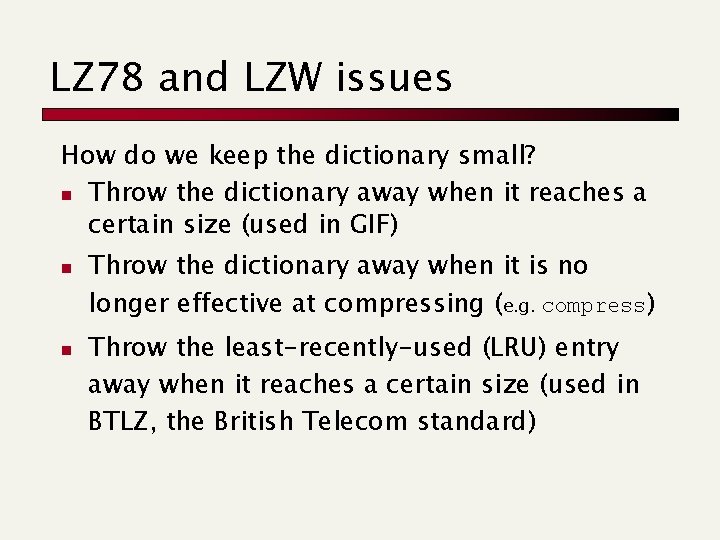
LZ 78 and LZW issues How do we keep the dictionary small? n Throw the dictionary away when it reaches a certain size (used in GIF) n n Throw the dictionary away when it is no longer effective at compressing (e. g. compress) Throw the least-recently-used (LRU) entry away when it reaches a certain size (used in BTLZ, the British Telecom standard)

You find this at: www. gzip. org/zlib/

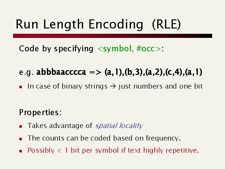
Run Length Encoding (RLE) Code by specifying <symbol, #occ>: e. g. abbbaacccca => (a, 1), (b, 3), (a, 2), (c, 4), (a, 1) n In case of binary strings just numbers and one bit Properties: n Takes advantage of spatial locality n The counts can be coded based on frequency. n Possibly < 1 bit per symbol if text highly repetitive.

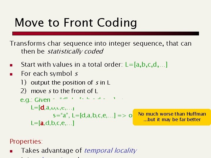
Move to Front Coding Transforms char sequence into integer sequence, that can then be statistically coded n n Start with values in a total order: L=[a, b, c, d, …] For each symbol s 1) output the position of s in L 2) move s to the front of L e. g. : Given s=“d”, L=[a, b, c, d, e, …] => out: 3, new L=[d, a, b, c, e, …] s=“a”, L=[d, a, b, c, e, …] => out: No 1, much newworse than Huffman. . . but it may be far better L=[a, d, b, c, e, …] Properties: n Takes advantage of temporal locality

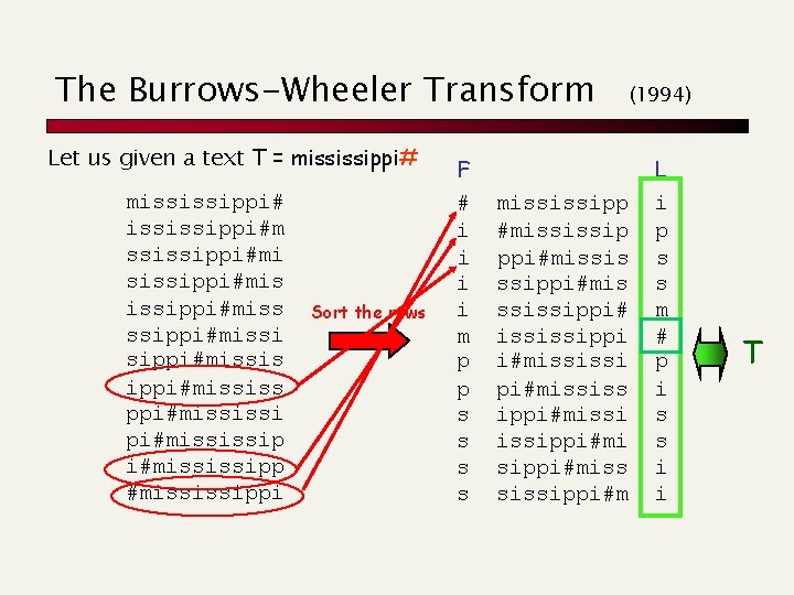
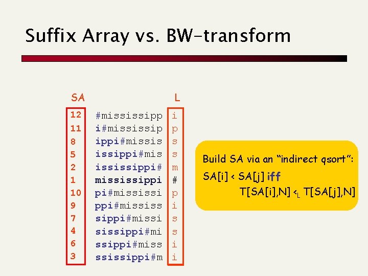
The Burrows-Wheeler Transform Let us given a text T = mississippi#m ssissippi#mis issippi#missi sippi#mississ ppi#mississip i#mississippi Sort the rows F # i i m p p s s (1994) mississipp #mississip ppi#missis ssippi#mis ssissippi# ississippi i#mississi pi#mississ ippi#missippi#mi sippi#miss sissippi#m L i p s s m # p i s s i i T

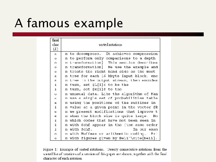
A famous example

Suffix Array vs. BW-transform SA 12 11 8 5 2 1 10 9 7 4 6 3 L #mississipp i#mississip ippi#missis issippi#mis ississippi# mississippi pi#mississi ppi#mississ sippi#missi sissippi#miss ssissippi#m i p s s m # p i s s i i Build SA via an “indirect qsort”: SA[i] < SA[j] iff T[SA[i], N] <L T[SA[j], N]

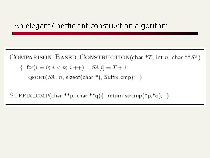
An elegant/inefficient construction algorithm

BWT construction: Manzini’s web page

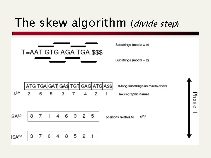
The skew algorithm (divide step)

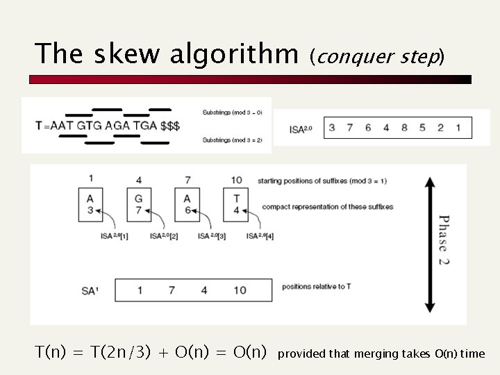
The skew algorithm T(n) = T(2 n/3) + O(n) = O(n) (conquer step) provided that merging takes O(n) time

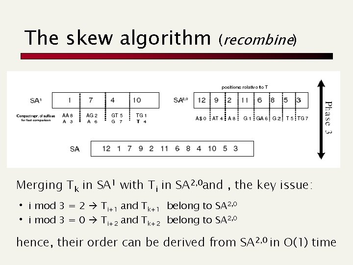
The skew algorithm (recombine) Merging Tk in SA 1 with Ti in SA 2, 0 and , the key issue: • i mod 3 = 2 Ti+1 and Tk+1 • i mod 3 = 0 Ti+2 and Tk+2 belong to SA 2, 0 hence, their order can be derived from SA 2, 0 in O(1) time

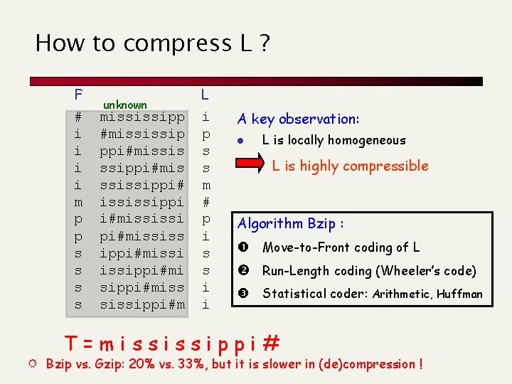
How to compress L ? F # i i m p p s s unknown mississipp #mississip ppi#missis ssippi#mis ssissippi# ississippi i#mississi pi#mississ ippi#missippi#mi sippi#miss sissippi#m L i p s s m # p i s s i i A key observation: l L is locally homogeneous L is highly compressible Algorithm Bzip : Move-to-Front coding of L Run-Length coding (Wheeler’s code) Statistical coder: Arithmetic, Huffman T=mississippi# R Bzip vs. Gzip: 20% vs. 33%, but it is slower in (de)compression !

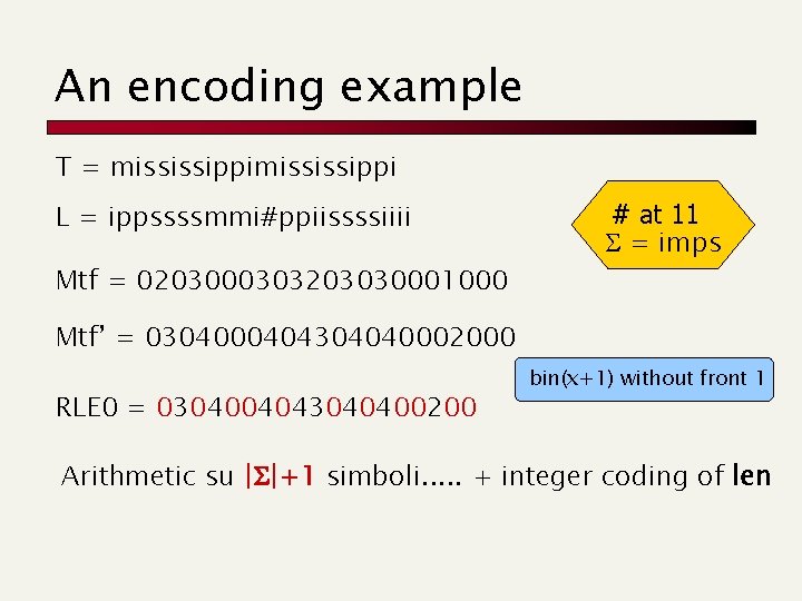
An encoding example T = mississippi L = ippssssmmi#ppiissssiiii Mtf = 0203000303203030001000 # at 11 = imps Mtf’ = 0304000404304040002000 RLE 0 = 0304004043040400200 bin(x+1) without front 1 Arithmetic su |S|+1 simboli. . . + integer coding of len

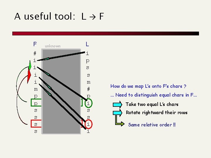
A useful tool: L F # i i m p p s s unknown mississipp #mississip ppi#missis ssippi#mis ssissippi# ississippi i#mississi pi#mississ ippi#missippi#mi sippi#miss sissippi#m L i p s s m # p i s s i i F How do we map L’s onto F’s chars ? . . . Need to distinguish equal chars in F. . . Take two equal L’s chars Rotate rightward their rows Same relative order !!

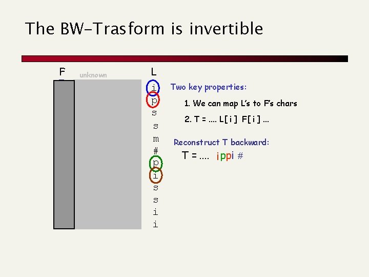
The BW-Trasform is invertible F # i i m p p s s unknown mississipp #mississip ppi#missis ssippi#mis ssissippi# ississippi i#mississi pi#mississ ippi#missippi#mi sippi#miss sissippi#m L i p s s m # p i s s i i Two key properties: 1. We can map L’s to F’s chars 2. T =. . L[ i ] F[ i ]. . . Reconstruct T backward: T =. . i ppi #

You find this at: sources. redhat. com/bzip 2/

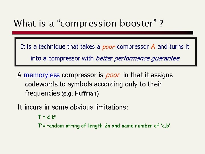
What is a “compression booster” ? It is a technique that takes a poor compressor A and turns it into a compressor with better performance guarantee A memoryless compressor is poor in that it assigns codewords to symbols according only to their frequencies (e. g. Huffman) It incurs in some obvious limitations: T = a n bn T’= random string of length 2 n and same number of ‘a, b’

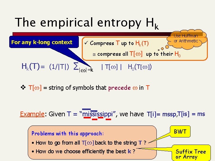
The empirical entropy Hk For any k-long context ü Compress T up to Hk(T) Use Huffman or Arithmetic compress all T[w] up to their H 0 Hk(T) = (1/|T|) ∑|w|=k | T[w] | H 0(T[w]) v T[w] = string of symbols that precede w in T Example: Given T = “mississippi”, we have T[i]= mssp, T[is] = ms Problems with this approach: BWT • How to go from all T[w] back to the string T ? • How do we choose efficiently the best k ? Suffix Tree or Array

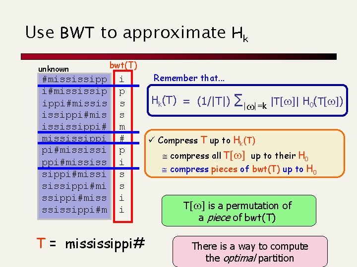
Use BWT to approximate Hk unknown #mississipp i#mississip ippi#missis issippi#mis ississippi# mississippi pi#mississi ppi#mississ sippi#missi sissippi#miss ssissippi#m bwt(T) i p s s m # p i s s i i T = mississippi# Remember that. . . Hk(T) = (1/|T|) ∑|w|=k |T[w]| H 0(T[w]) ü Compress T up to Hk(T) compress all T[w] up to their H 0 compress pieces of bwt(T) up to H 0 T[w] is a permutation of a piece of bwt(T) There is a way to compute the optimal partition

You find this at Manzini’s home page