Information Retrieval and Web Search Lecture 13 Nave

Information Retrieval and Web Search Lecture 13: Naïve Bayes. Text Classification

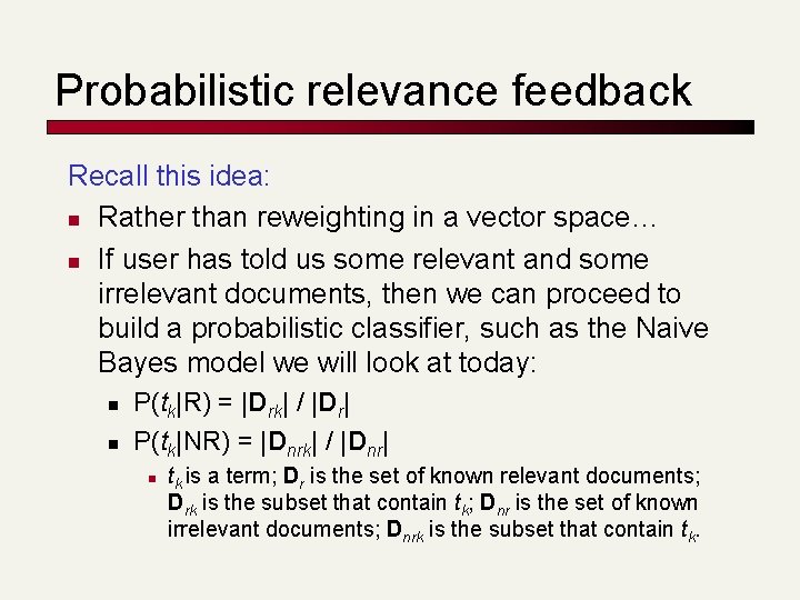
Probabilistic relevance feedback Recall this idea: n Rather than reweighting in a vector space… n If user has told us some relevant and some irrelevant documents, then we can proceed to build a probabilistic classifier, such as the Naive Bayes model we will look at today: n n P(tk|R) = |Drk| / |Dr| P(tk|NR) = |Dnrk| / |Dnr| n tk is a term; Dr is the set of known relevant documents; Drk is the subset that contain tk; Dnr is the set of known irrelevant documents; Dnrk is the subset that contain tk.

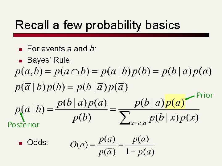
Recall a few probability basics n n For events a and b: Bayes’ Rule Prior Posterior n Odds:

Text classification: Naïve Bayes Text Classification n Today: n n n Introduction to Text Classification Probabilistic Language Models Naïve Bayes text categorization

Is this spam? From: "" <takworlld@hotmail. com> Subject: real estate is the only way. . . gem oalvgkay Anyone can buy real estate with no money down Stop paying rent TODAY ! There is no need to spend hundreds or even thousands for similar courses I am 22 years old and I have already purchased 6 properties using the methods outlined in this truly INCREDIBLE ebook. Change your life NOW ! ========================= Click Below to order: http: //www. wholesaledaily. com/sales/nmd. htm =========================

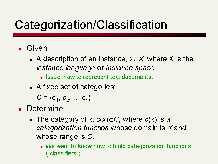
Categorization/Classification n Given: n A description of an instance, x X, where X is the instance language or instance space. n n n Issue: how to represent text documents. A fixed set of categories: C = {c 1, c 2, …, cn} Determine: n The category of x: c(x) C, where c(x) is a categorization function whose domain is X and whose range is C. n We want to know how to build categorization functions (“classifiers”).

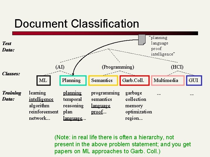
Document Classification “planning language proof intelligence” Test Data: (AI) (Programming) (HCI) Classes: ML Training Data: learning intelligence algorithm reinforcement network. . . Planning Semantics planning temporal reasoning plan language. . . programming semantics language proof. . . Garb. Coll. Multimedia garbage. . . collection memory optimization region. . . GUI. . . (Note: in real life there is often a hierarchy, not present in the above problem statement; and you get papers on ML approaches to Garb. Coll. )

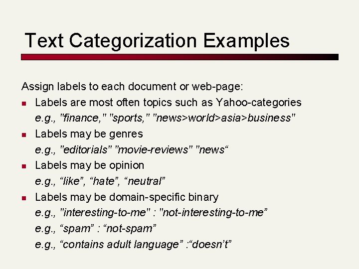
Text Categorization Examples Assign labels to each document or web-page: n Labels are most often topics such as Yahoo-categories e. g. , "finance, " "sports, " "news>world>asia>business" n Labels may be genres e. g. , "editorials" "movie-reviews" "news“ n Labels may be opinion e. g. , “like”, “hate”, “neutral” n Labels may be domain-specific binary e. g. , "interesting-to-me" : "not-interesting-to-me” e. g. , “spam” : “not-spam” e. g. , “contains adult language” : “doesn’t”

Classification Methods (1) n Manual classification n n Used by Yahoo!, Looksmart, about. com, ODP, Medline Very accurate when job is done by experts Consistent when the problem size and team is small Difficult and expensive to scale

Classification Methods (2) n Automatic document classification n Hand-coded rule-based systems n n n One technique used by CS dept’s spam filter, Reuters, CIA, Verity, … E. g. , assign category if document contains a given boolean combination of words Standing queries: Commercial systems have complex query languages (everything in IR query languages + accumulators) Accuracy is often very high if a rule has been carefully refined over time by a subject expert Building and maintaining these rules is expensive

Classification Methods (3) n Supervised learning of a document-label assignment function n Many systems partly rely on machine learning (Autonomy, MSN, Verity, Enkata, Yahoo!, …) n n n n k-Nearest Neighbors (simple, powerful) Naive Bayes (simple, common method) Support-vector machines (new, more powerful) … plus many other methods No free lunch: requires hand-classified training data But data can be built up (and refined) by amateurs Note that many commercial systems use a mixture of methods

Bayesian Methods n n n Our focus this lecture Learning and classification methods based on probability theory. Bayes theorem plays a critical role in probabilistic learning and classification. Build a generative model that approximates how data is produced Uses prior probability of each category given no information about an item. Categorization produces a posterior probability distribution over the possible categories given a description of an item.

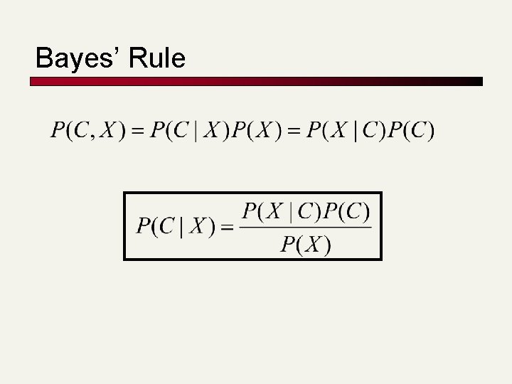
Bayes’ Rule

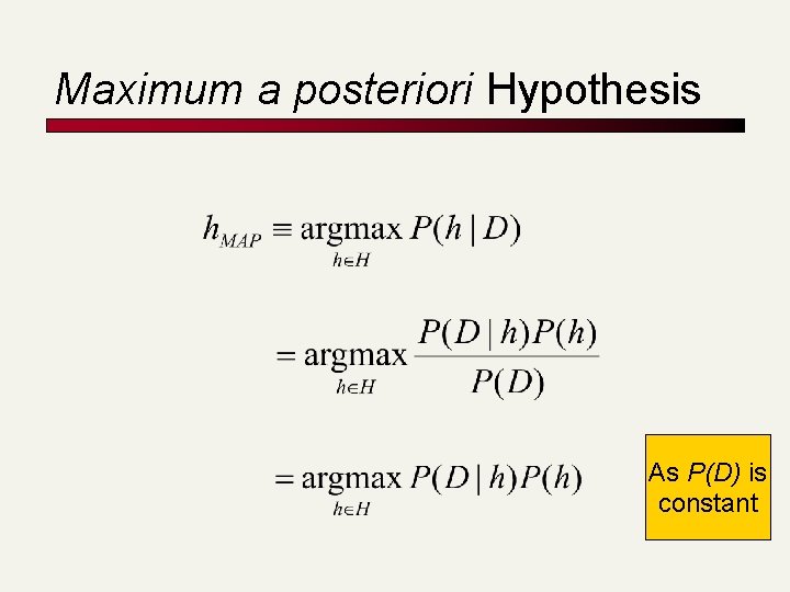
Maximum a posteriori Hypothesis As P(D) is constant

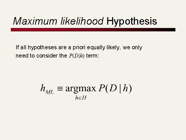
Maximum likelihood Hypothesis If all hypotheses are a priori equally likely, we only need to consider the P(D|h) term:

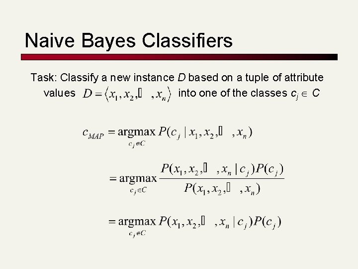
Naive Bayes Classifiers Task: Classify a new instance D based on a tuple of attribute values into one of the classes cj C

Naïve Bayes Classifier: Naïve Bayes Assumption n P(cj) n n Can be estimated from the frequency of classes in the training examples. P(x 1, x 2, …, xn|cj) n n O(|X|n • |C|) parameters Could only be estimated if a very, very large number of training examples was available. Naïve Bayes Conditional Independence Assumption: n Assume that the probability of observing the conjunction of attributes is equal to the product of the individual probabilities P(xi|cj).

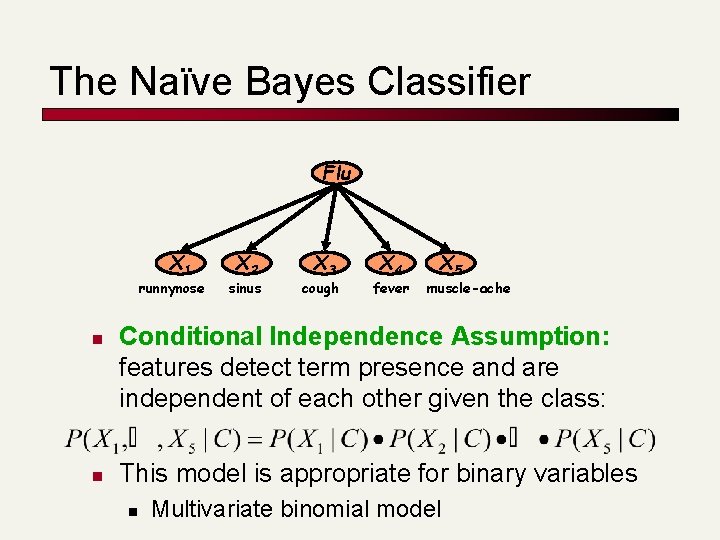
The Naïve Bayes Classifier Flu X 1 runnynose n n X 2 sinus X 3 cough X 4 fever X 5 muscle-ache Conditional Independence Assumption: features detect term presence and are independent of each other given the class: This model is appropriate for binary variables n Multivariate binomial model

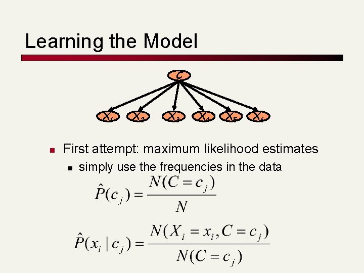
Learning the Model C X 1 n X 2 X 3 X 4 X 5 X 6 First attempt: maximum likelihood estimates n simply use the frequencies in the data

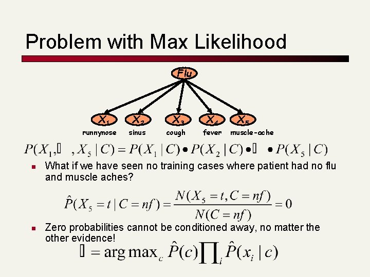
Problem with Max Likelihood Flu X 1 runnynose n n X 2 sinus X 3 cough X 4 fever X 5 muscle-ache What if we have seen no training cases where patient had no flu and muscle aches? Zero probabilities cannot be conditioned away, no matter the other evidence!

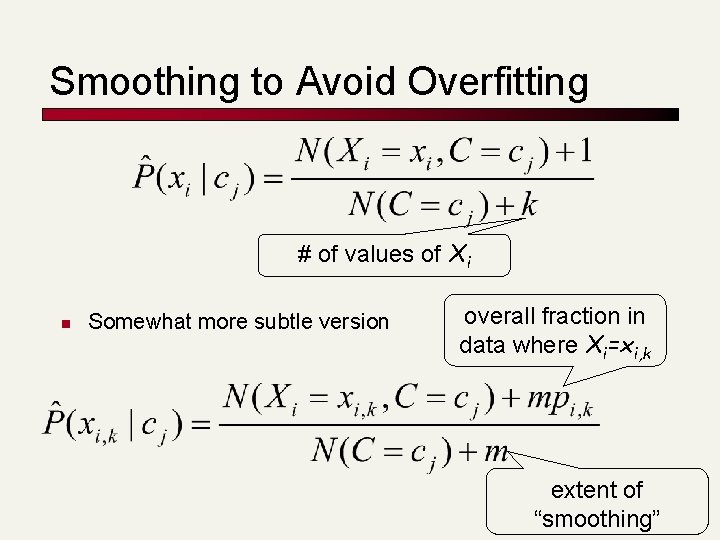
Smoothing to Avoid Overfitting # of values of Xi n Somewhat more subtle version overall fraction in data where Xi=xi, k extent of “smoothing”

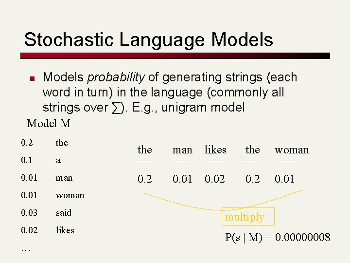
Stochastic Language Models n Models probability of generating strings (each word in turn) in the language (commonly all strings over ∑). E. g. , unigram model M 0. 2 the 0. 1 a 0. 01 man 0. 01 woman 0. 03 said 0. 02 likes … the man likes the woman 0. 2 0. 01 0. 02 0. 01 multiply P(s | M) = 0. 00000008

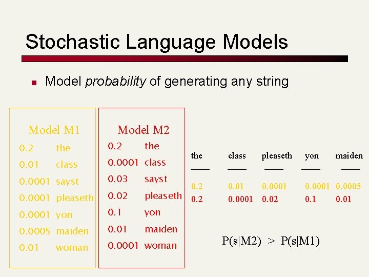
Stochastic Language Models n Model probability of generating any string Model M 1 0. 2 0. 01 Model M 2 the 0. 2 the class 0. 0001 sayst 0. 03 0. 0001 pleaseth 0. 02 0. 0001 yon 0. 1 0. 2 pleaseth 0. 2 yon 0. 0005 maiden 0. 01 0. 0001 woman sayst the class pleaseth 0. 01 0. 0001 0. 02 yon maiden 0. 0001 0. 0005 0. 1 0. 01 P(s|M 2) > P(s|M 1)

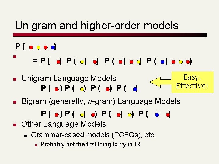
Unigram and higher-order models P( n n ) =P( ) P( | Unigram Language Models P( ) P( | ) Easy. Effective! ) n Bigram (generally, n-gram) Language Models n P( )P( | ) P( Other Language Models n | ) P( Grammar-based models (PCFGs), etc. n Probably not the first thing to try in IR | )

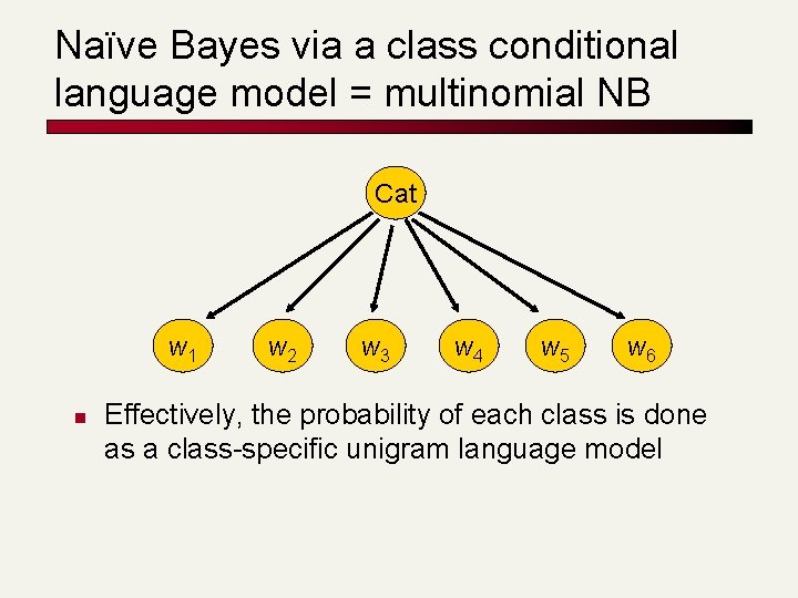
Naïve Bayes via a class conditional language model = multinomial NB Cat w 1 n w 2 w 3 w 4 w 5 w 6 Effectively, the probability of each class is done as a class-specific unigram language model

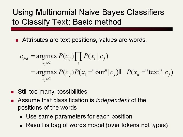
Using Multinomial Naive Bayes Classifiers to Classify Text: Basic method n n n Attributes are text positions, values are words. Still too many possibilities Assume that classification is independent of the positions of the words n Use same parameters for each position n Result is bag of words model (over tokens not types)

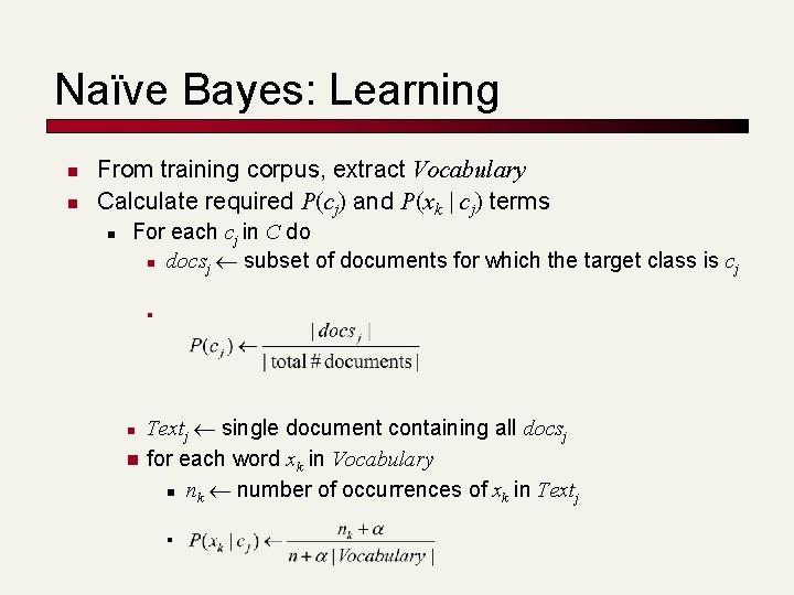
Naïve Bayes: Learning n n From training corpus, extract Vocabulary Calculate required P(cj) and P(xk | cj) terms n For each cj in C do n docsj subset of documents for which the target class is cj n Textj single document containing all docsj n for each word xk in Vocabulary n nk number of occurrences of xk in Textj n n

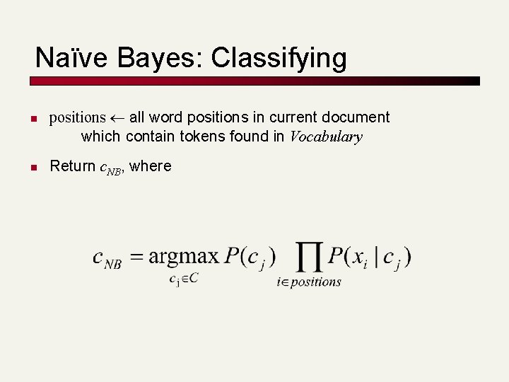
Naïve Bayes: Classifying n n positions all word positions in current document which contain tokens found in Vocabulary Return c. NB, where

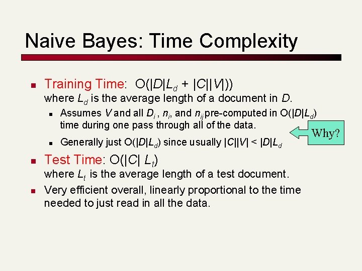
Naive Bayes: Time Complexity n Training Time: O(|D|Ld + |C||V|)) where Ld is the average length of a document in D. n n Assumes V and all Di , ni, and nij pre-computed in O(|D|Ld) time during one pass through all of the data. Generally just O(|D|Ld) since usually |C||V| < |D|Ld Test Time: O(|C| Lt) where Lt is the average length of a test document. Very efficient overall, linearly proportional to the time needed to just read in all the data. Why?

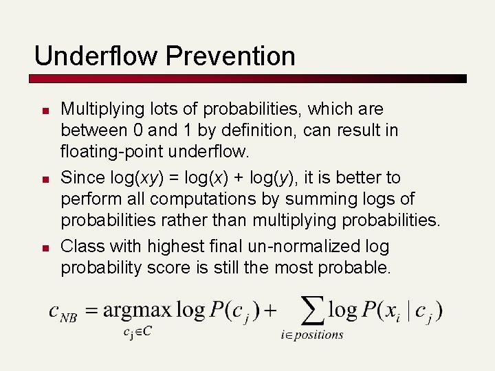
Underflow Prevention n Multiplying lots of probabilities, which are between 0 and 1 by definition, can result in floating-point underflow. Since log(xy) = log(x) + log(y), it is better to perform all computations by summing logs of probabilities rather than multiplying probabilities. Class with highest final un-normalized log probability score is still the most probable.

Note: Two Models n Model 1: Multivariate binomial n n n One feature Xw for each word in dictionary Xw = true in document d if w appears in d Naive Bayes assumption: n n Given the document’s topic, appearance of one word in the document tells us nothing about chances that another word appears This is the model used in the binary independence model in classic probabilistic relevance feedback in hand-classified data (Maron in IR was a very early user of NB)

Two Models n Model 2: Multinomial = Class conditional unigram n One feature Xi for each word pos in document n n n Value of Xi is the word in position i Naïve Bayes assumption: n n feature’s values are all words in dictionary Given the document’s topic, word in one position in the document tells us nothing about words in other positions Second assumption: n Word appearance does not depend on position for all positions i, j, word w, and class c n Just have one multinomial feature predicting all words

Parameter estimation n Binomial model: fraction of documents of topic cj in which word w appears n Multinomial model: fraction of times in which word w appears across all documents of topic cj n n Can create a mega-document for topic j by concatenating all documents in this topic Use frequency of w in mega-document

Classification n Multinomial vs Multivariate binomial? n Multinomial is in general better n See results figures later

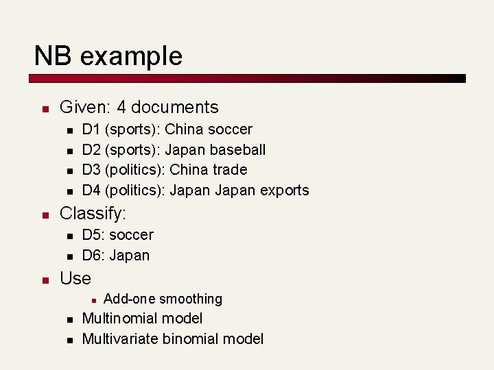
NB example n Given: 4 documents n n n Classify: n n n D 1 (sports): China soccer D 2 (sports): Japan baseball D 3 (politics): China trade D 4 (politics): Japan exports D 5: soccer D 6: Japan Use n n n Add-one smoothing Multinomial model Multivariate binomial model

Feature Selection: Why? n Text collections have a large number of features n n May make using a particular classifier feasible n n Some classifiers can’t deal with 100, 000 of features Reduces training time n n 10, 000 – 1, 000 unique words … and more Training time for some methods is quadratic or worse in the number of features Can improve generalization (performance) n n Eliminates noise features Avoids overfitting

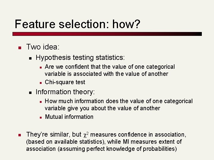
Feature selection: how? n Two idea: n Hypothesis testing statistics: n n n Information theory: n n n Are we confident that the value of one categorical variable is associated with the value of another Chi-square test How much information does the value of one categorical variable give you about the value of another Mutual information They’re similar, but 2 measures confidence in association, (based on available statistics), while MI measures extent of association (assuming perfect knowledge of probabilities)

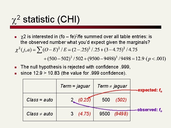
2 statistic (CHI) n n n 2 is interested in (fo – fe)2/fe summed over all table entries: is the observed number what you’d expect given the marginals? The null hypothesis is rejected with confidence. 999, since 12. 9 > 10. 83 (the value for. 999 confidence). Term = jaguar Class = auto Class auto 2 (0. 25) 3 (4. 75) Term jaguar 500 expected: fe (502) 9500 (9498) observed: fo

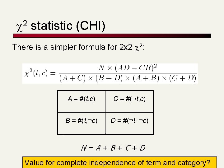
2 statistic (CHI) There is a simpler formula for 2 x 2 2: A = #(t, c) C = #(¬t, c) B = #(t, ¬c) D = #(¬t, ¬c) N=A+B+C+D Value for complete independence of term and category?

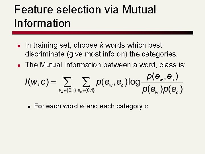
Feature selection via Mutual Information n n In training set, choose k words which best discriminate (give most info on) the categories. The Mutual Information between a word, class is: n For each word w and each category c

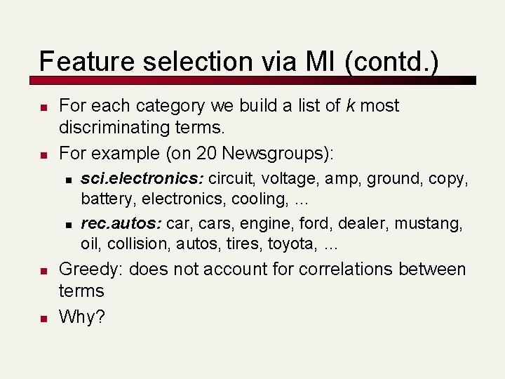
Feature selection via MI (contd. ) n n For each category we build a list of k most discriminating terms. For example (on 20 Newsgroups): n n sci. electronics: circuit, voltage, amp, ground, copy, battery, electronics, cooling, … rec. autos: car, cars, engine, ford, dealer, mustang, oil, collision, autos, tires, toyota, … Greedy: does not account for correlations between terms Why?

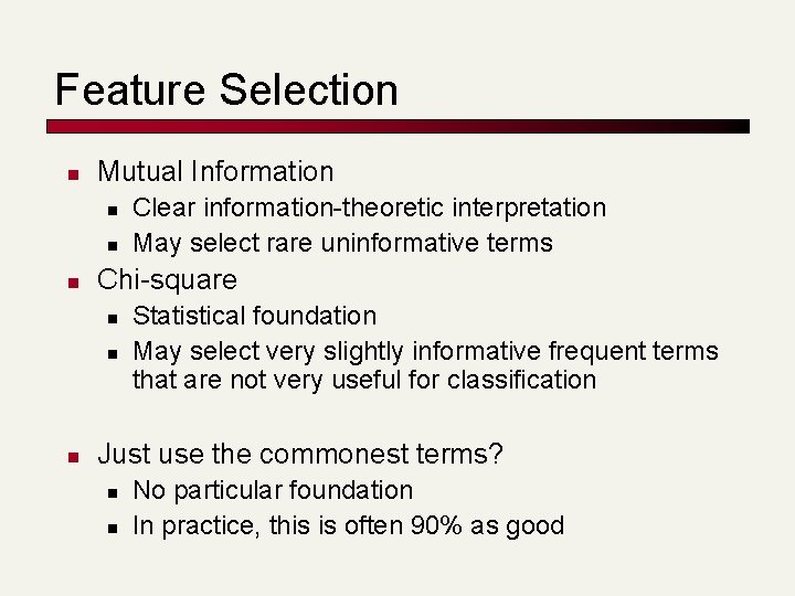
Feature Selection n Mutual Information n Chi-square n n n Clear information-theoretic interpretation May select rare uninformative terms Statistical foundation May select very slightly informative frequent terms that are not very useful for classification Just use the commonest terms? n n No particular foundation In practice, this is often 90% as good

Feature selection for NB n n n In general feature selection is necessary for binomial NB. Otherwise you suffer from noise, multi-counting “Feature selection” really means something different for multinomial NB. It means dictionary truncation n n The multinomial NB model only has 1 feature This “feature selection” normally isn’t needed for multinomial NB, but may help a fraction with quantities that are badly estimated

Evaluating Categorization n n Evaluation must be done on test data that are independent of the training data (usually a disjoint set of instances). Classification accuracy: c/n where n is the total number of test instances and c is the number of test instances correctly classified by the system. Results can vary based on sampling error due to different training and test sets. Average results over multiple training and test sets (splits of the overall data) for the best results.

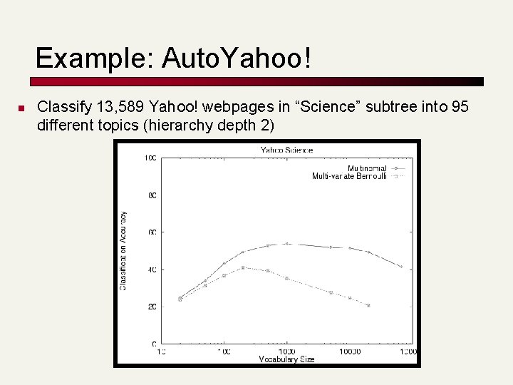
Example: Auto. Yahoo! n Classify 13, 589 Yahoo! webpages in “Science” subtree into 95 different topics (hierarchy depth 2)

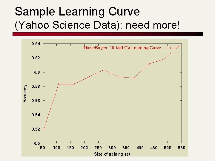
Sample Learning Curve (Yahoo Science Data): need more!

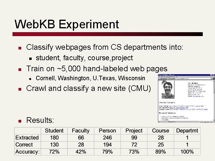
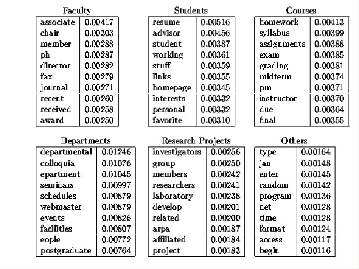
Web. KB Experiment n Classify webpages from CS departments into: n n student, faculty, course, project Train on ~5, 000 hand-labeled web pages n Cornell, Washington, U. Texas, Wisconsin n Crawl and classify a new site (CMU) n Results:

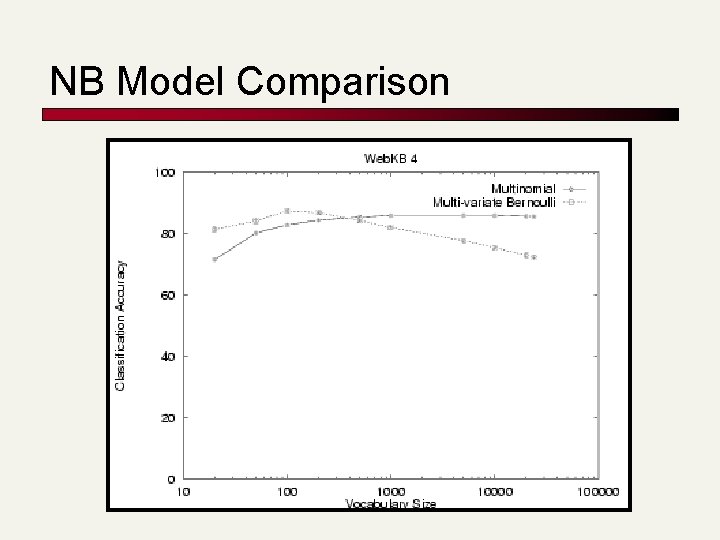
NB Model Comparison

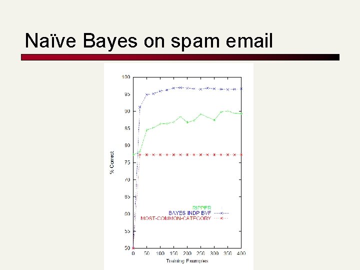
Naïve Bayes on spam email

Spam. Assassin n Naïve Bayes has found a home for spam filtering n Graham’s A Plan for Spam n n n Naive Bayes-like classifier with weird parameter estimation Widely used in spam filters n n n And its mutant offspring. . . Classic Naive Bayes superior when appropriately used According to David D. Lewis Many email filters use NB classifiers n But also many other things: black hole lists, etc.

Violation of NB Assumptions n n n Conditional independence “Positional independence” Examples?

Naïve Bayes Posterior Probabilities n n Classification results of naïve Bayes (the class with maximum posterior probability) are usually fairly accurate. However, due to the inadequacy of the conditional independence assumption, the actual posterior-probability numerical estimates are not. n Output probabilities are generally very close to 0 or 1.

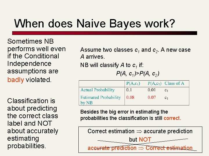
When does Naive Bayes work? Sometimes NB performs well even if the Conditional Independence assumptions are badly violated. Classification is about predicting the correct class label and NOT about accurately estimating probabilities. Assume two classes c 1 and c 2. A new case A arrives. NB will classify A to c 1 if: P(A, c 1)>P(A, c 2) Besides the big error in estimating the probabilities the classification is still correct. Correct estimation accurate prediction but NOT accurate prediction Correct estimation

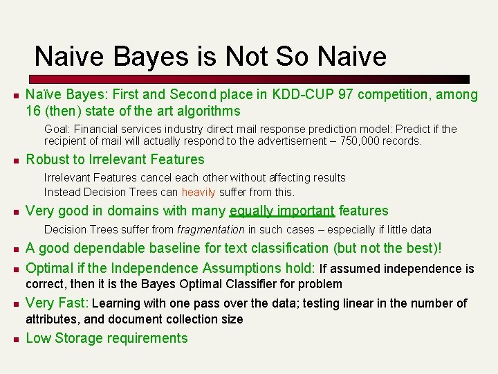
Naive Bayes is Not So Naive n Naïve Bayes: First and Second place in KDD-CUP 97 competition, among 16 (then) state of the art algorithms Goal: Financial services industry direct mail response prediction model: Predict if the recipient of mail will actually respond to the advertisement – 750, 000 records. n Robust to Irrelevant Features cancel each other without affecting results Instead Decision Trees can heavily suffer from this. n Very good in domains with many equally important features Decision Trees suffer from fragmentation in such cases – especially if little data n n A good dependable baseline for text classification (but not the best)! Optimal if the Independence Assumptions hold: If assumed independence is correct, then it is the Bayes Optimal Classifier for problem n Very Fast: Learning with one pass over the data; testing linear in the number of attributes, and document collection size n Low Storage requirements

Resources n n IIR 13 Fabrizio Sebastiani. Machine Learning in Automated Text Categorization. ACM Computing Surveys, 34(1): 1 -47, 2002. Andrew Mc. Callum and Kamal Nigam. A Comparison of Event Models for Naive Bayes Text Classification. In AAAI/ICML-98 Workshop on Learning for Text Categorization, pp. 41 -48. Tom Mitchell, Machine Learning. Mc. Graw-Hill, 1997. n n Clear simple explanation Yiming Yang & Xin Liu, A re-examination of text categorization methods. Proceedings of SIGIR, 1999.