Information Management Information Retrieval hussein suleman uct cs

Information Management Information Retrieval hussein suleman uct cs 303 2004

Introduction Information retrieval is the process of locating the most relevant information to satisfy a specific information need. p Traditionally, we used databases and keywords to locate information. p The most common modern application is search engines. p Historically, the technology has been developed from the mid-50’s onwards, with a lot of fundamental research conducted pre-Internet! p

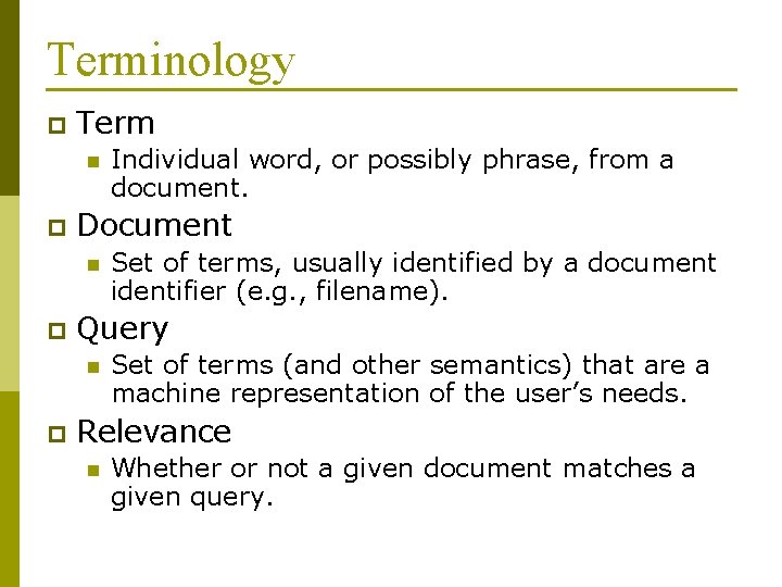
Terminology p Term n p Document n p Set of terms, usually identified by a document identifier (e. g. , filename). Query n p Individual word, or possibly phrase, from a document. Set of terms (and other semantics) that are a machine representation of the user’s needs. Relevance n Whether or not a given document matches a given query.

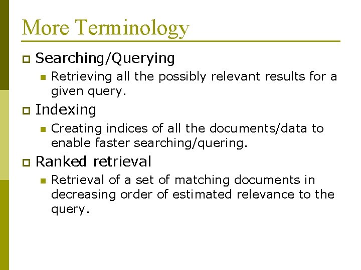
More Terminology p Searching/Querying n p Indexing n p Retrieving all the possibly relevant results for a given query. Creating indices of all the documents/data to enable faster searching/quering. Ranked retrieval n Retrieval of a set of matching documents in decreasing order of estimated relevance to the query.

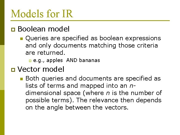
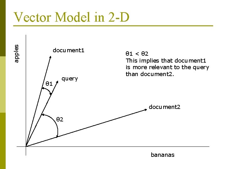
Models for IR p Boolean model n Queries are specified as boolean expressions and only documents matching those criteria are returned. p p e. g. , apples AND bananas Vector model n Both queries and documents are specified as lists of terms and mapped into an ndimensional space (where n is the number of possible terms). The relevance then depends on the angle between the vectors.

apples Vector Model in 2 -D document 1 θ 1 query θ 1 < θ 2 This implies that document 1 is more relevant to the query than document 2 θ 2 bananas

Extended Boolean Models p Any modern search engine that returns no results for a very long query probably uses some form of boolean model! n n p Altavista, Google, etc. Vector models are not as efficient as boolean models. Some extended boolean models filter on the basis of boolean matching and rank on the basis of term weights (tf. idf).

Filtering and Ranking p Filtering n n p Removal of non-relevant results. Filtering restricts the number of results to those that are probably relevant. Ranking n n Ordering of results according to calculated probability of relevance. Ranking puts the most probably relevant results at the “top of the list”.

Efficient Ranking Comparing every document to each query is very slow. p Use inverted files to speed up ranking algorithms by possibly ignoring: p n n p terms with zero occurrence in each documents where terms have a very low occurrence value. We are only interested in those documents that contain the terms in the query.

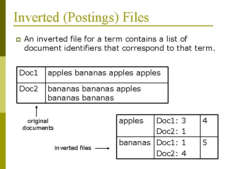
Inverted (Postings) Files p An inverted file for a term contains a list of document identifiers that correspond to that term. Doc 1 apples bananas apples Doc 2 bananas apples original documents inverted files Doc 1: 3 Doc 2: 1 4 bananas Doc 1: 1 Doc 2: 4 5

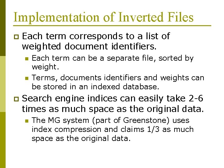
Implementation of Inverted Files p Each term corresponds to a list of weighted document identifiers. n n p Each term can be a separate file, sorted by weight. Terms, documents identifiers and weights can be stored in an indexed database. Search engine indices can easily take 2 -6 times as much space as the original data. n The MG system (part of Greenstone) uses index compression and claims 1/3 as much space as the original data.

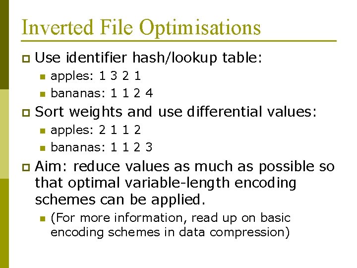
Inverted File Optimisations p Use identifier hash/lookup table: n n p Sort weights and use differential values: n n p apples: 1 3 2 1 bananas: 1 1 2 4 apples: 2 1 1 2 bananas: 1 1 2 3 Aim: reduce values as much as possible so that optimal variable-length encoding schemes can be applied. n (For more information, read up on basic encoding schemes in data compression)

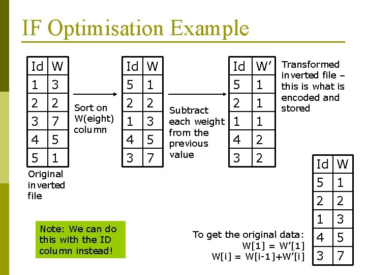
IF Optimisation Example Id 1 2 3 W 3 2 7 4 5 5 1 Sort on W(eight) column Id 5 2 1 W 1 2 3 4 3 5 7 Subtract each weight from the previous value Id 5 2 1 W’ 1 1 1 4 3 2 2 Transformed inverted file – this is what is encoded and stored Original inverted file Note: We can do this with the ID column instead! To get the original data: W[1] = W’[1] W[i] = W[i-1]+W’[i] Id 5 2 1 W 1 2 3 4 3 5 7

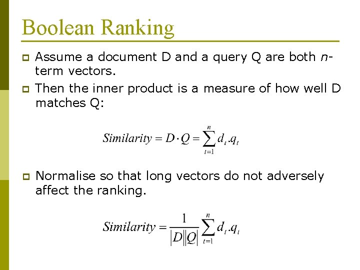
Boolean Ranking p p p Assume a document D and a query Q are both nterm vectors. Then the inner product is a measure of how well D matches Q: Normalise so that long vectors do not adversely affect the ranking.

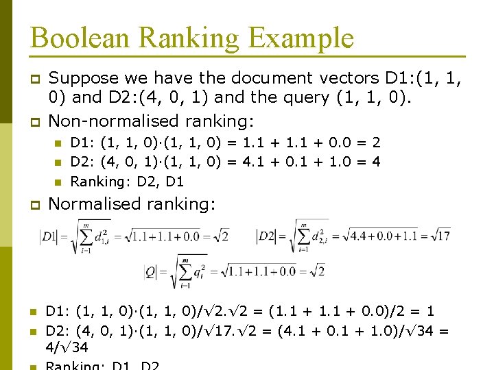
Boolean Ranking Example p p Suppose we have the document vectors D 1: (1, 1, 0) and D 2: (4, 0, 1) and the query (1, 1, 0). Non-normalised ranking: n n n D 1: (1, 1, 0)·(1, 1, 0) = 1. 1 + 0. 0 = 2 D 2: (4, 0, 1)·(1, 1, 0) = 4. 1 + 0. 1 + 1. 0 = 4 Ranking: D 2, D 1 p Normalised ranking: n D 1: (1, 1, 0)·(1, 1, 0)/√ 2. √ 2 = (1. 1 + 0. 0)/2 = 1 D 2: (4, 0, 1)·(1, 1, 0)/√ 17. √ 2 = (4. 1 + 0. 1 + 1. 0)/√ 34 = 4/√ 34 n

tf. idf p Term frequency (tf) n p Document frequency (df) n p The number of occurrences of a term in a document – terms which occur more often in a document have higher tf. The number of documents a term occurs in – popular terms have a higher df. In general, terms with high “tf” and low “df” are good at describing a document and discriminating it from other documents – hence tf. idf (term frequency * inverse document frequency).

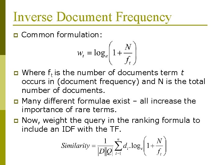
Inverse Document Frequency p Common formulation: p Where ft is the number of documents term t occurs in (document frequency) and N is the total number of documents. Many different formulae exist – all increase the importance of rare terms. Now, weight the query in the ranking formula to include an IDF with the TF. p p

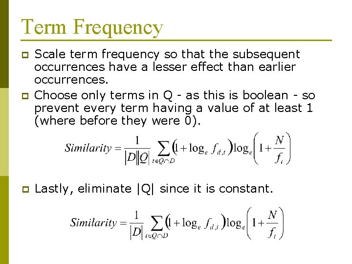
Term Frequency p p p Scale term frequency so that the subsequent occurrences have a lesser effect than earlier occurrences. Choose only terms in Q - as this is boolean - so prevent every term having a value of at least 1 (where before they were 0). Lastly, eliminate |Q| since it is constant.

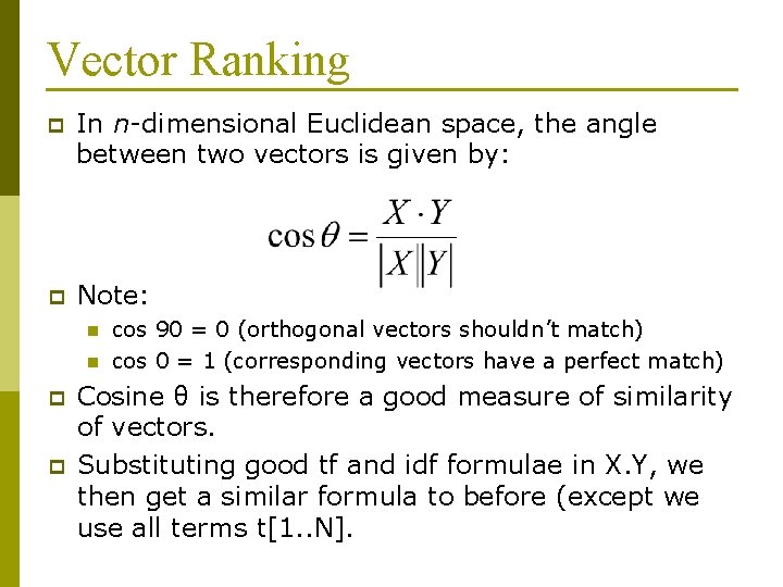
Vector Ranking p In n-dimensional Euclidean space, the angle between two vectors is given by: p Note: n n p p cos 90 = 0 (orthogonal vectors shouldn’t match) cos 0 = 1 (corresponding vectors have a perfect match) Cosine θ is therefore a good measure of similarity of vectors. Substituting good tf and idf formulae in X. Y, we then get a similar formula to before (except we use all terms t[1. . N].

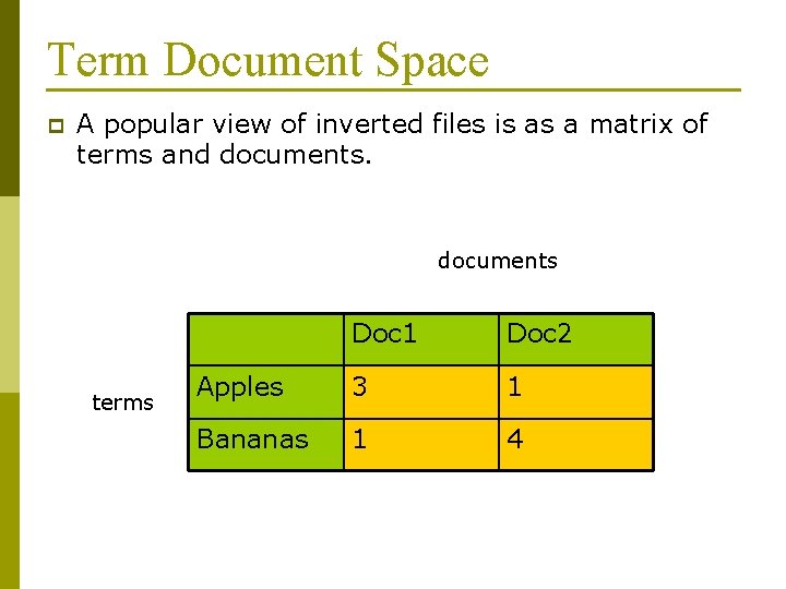
Term Document Space p A popular view of inverted files is as a matrix of terms and documents terms Doc 1 Doc 2 Apples 3 1 Bananas 1 4

Clustering In term-document space, documents that are similar will have vectors that are “close together”. p Even if a specific term of a query does not match a specific document, the clustering effect will compensate. p Centroids of the clusters can be used as cluster summaries. p Explicit clustering can be used to reduce the amount of information in T-D space. p

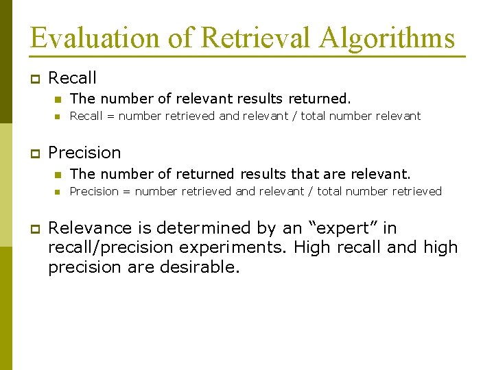
Evaluation of Retrieval Algorithms p p p Recall n The number of relevant results returned. n Recall = number retrieved and relevant / total number relevant Precision n The number of returned results that are relevant. n Precision = number retrieved and relevant / total number retrieved Relevance is determined by an “expert” in recall/precision experiments. High recall and high precision are desirable.

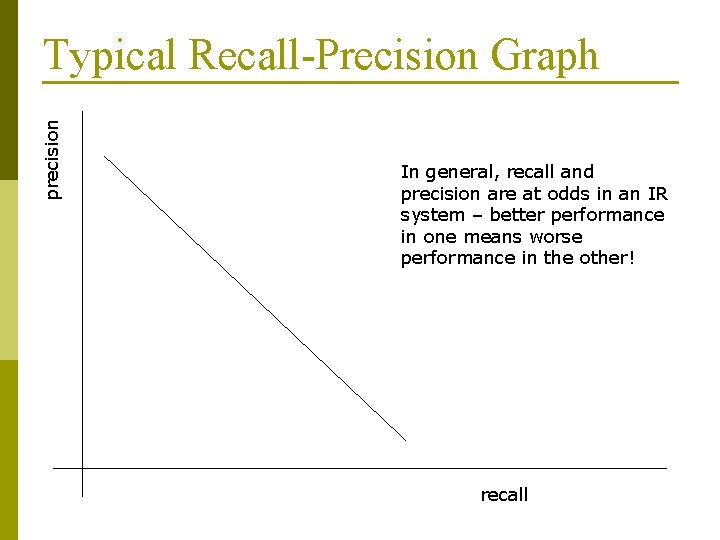
precision Typical Recall-Precision Graph In general, recall and precision are at odds in an IR system – better performance in one means worse performance in the other! recall

Other Techniques to Improve IR Stemming, Stopping p Thesauri p Metadata vs. Fulltext p Relevance Feedback p Inference Engines p LSI p Page. Rank p HITS p

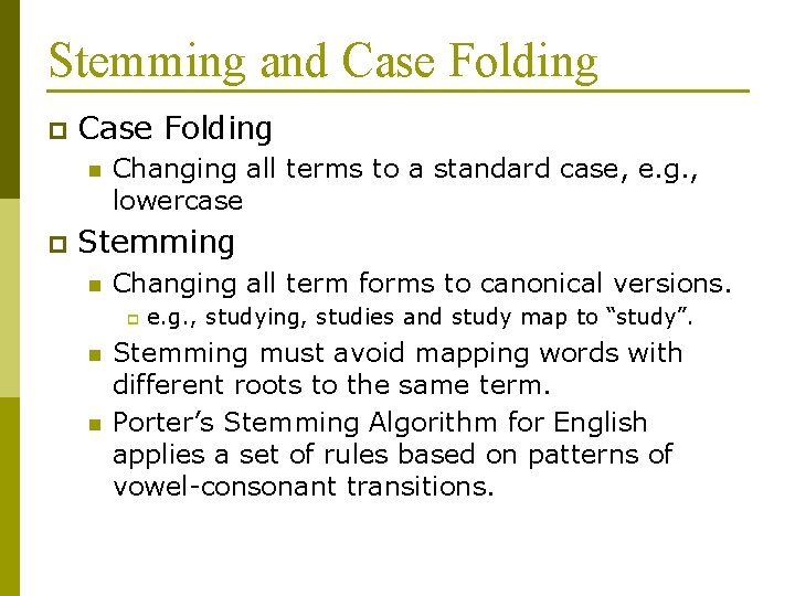
Stemming and Case Folding p Case Folding n p Changing all terms to a standard case, e. g. , lowercase Stemming n Changing all term forms to canonical versions. p n n e. g. , studying, studies and study map to “study”. Stemming must avoid mapping words with different roots to the same term. Porter’s Stemming Algorithm for English applies a set of rules based on patterns of vowel-consonant transitions.

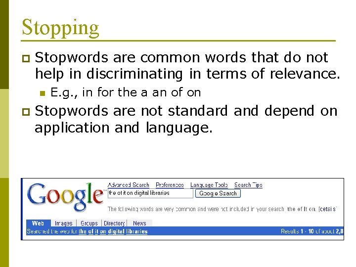
Stopping p Stopwords are common words that do not help in discriminating in terms of relevance. n p E. g. , in for the a an of on Stopwords are not standard and depend on application and language.

Thesauri p A thesaurus is a collection of words and their synonyms. n e. g. , According to Merriam-Webster, the synonyms for “library” are “archive” and “athenaeum”. An IR system can include all synonyms of a word to increase recall, but at a lower precision. p Thesauri can also be used for crosslanguage retrieval. p

Metadata vs. Full-text Text documents can be indexed by their contents or by their metadata. p Metadata indexing is faster and uses less storage. p Metadata can be obtained more easily (e. g. , using open standards) while full text is often restricted. p Full-text indexing does not rely on good quality metadata and can find very specific pieces of information. p

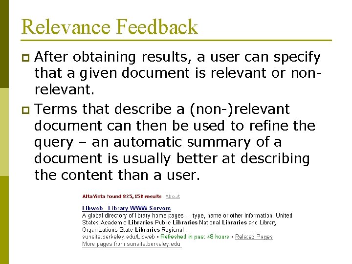
Relevance Feedback After obtaining results, a user can specify that a given document is relevant or nonrelevant. p Terms that describe a (non-)relevant document can then be used to refine the query – an automatic summary of a document is usually better at describing the content than a user. p

Inference Engines p Machine learning can be used to digest a document collection and perform query matching. n n p Connectionist models (e. g. , neural networks) Decision trees (e. g. , C 5) Combined with traditional statistical approaches, this can result in increased recall/precision.

Latent Semantic Indexing LSI is a technique to reduce the dimensionality of the term-document space, resulting in greater speed and arguably better results. p Problems with traditional approach: p n n p Synonymy – two different words that mean the same thing. Polysemy – two different meanings for a single word. LSI addresses both of these problems by transforming data to its “latent semantics. ”

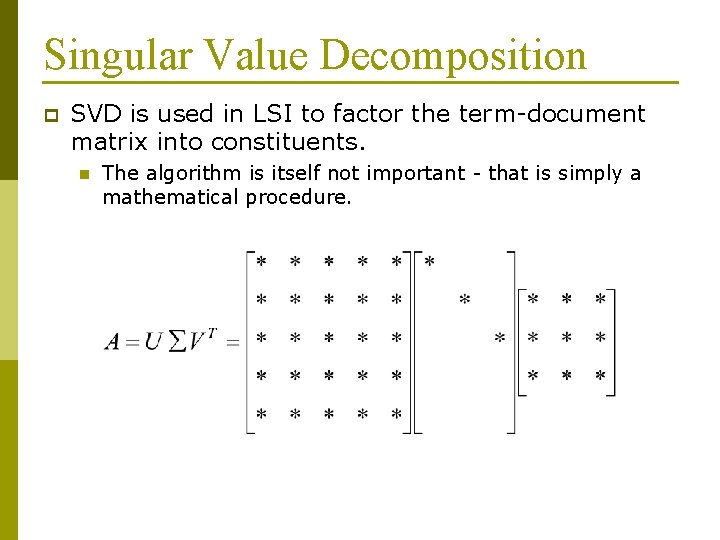
Singular Value Decomposition p SVD is used in LSI to factor the term-document matrix into constituents. n The algorithm is itself not important - that is simply a mathematical procedure.

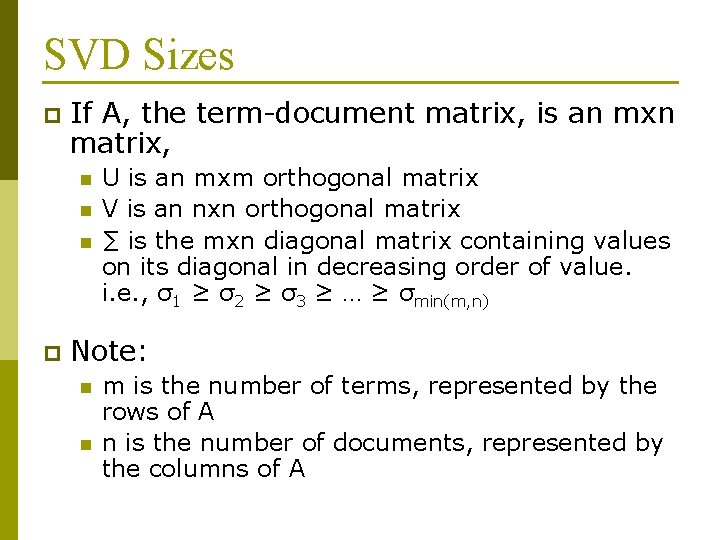
SVD Sizes p If A, the term-document matrix, is an mxn matrix, n n n p U is an mxm orthogonal matrix V is an nxn orthogonal matrix ∑ is the mxn diagonal matrix containing values on its diagonal in decreasing order of value. i. e. , σ1 ≥ σ2 ≥ σ3 ≥ … ≥ σmin(m, n) Note: n n m is the number of terms, represented by the rows of A n is the number of documents, represented by the columns of A

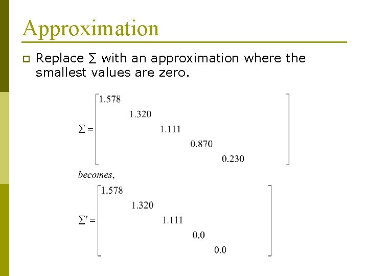
Approximation p Replace ∑ with an approximation where the smallest values are zero.

Advantages of LSI Smaller vectors – faster query matching. p Smaller term-document space – less storage required. p Automatic clustering of documents based on mathematical similarity (basis vector calculations). p Elimination of “noise” in document collection. p

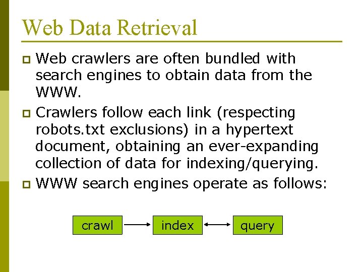
Web Data Retrieval Web crawlers are often bundled with search engines to obtain data from the WWW. p Crawlers follow each link (respecting robots. txt exclusions) in a hypertext document, obtaining an ever-expanding collection of data for indexing/querying. p WWW search engines operate as follows: p crawl index query

Page. Rank (popularised by Google) determines the rank of a document based on the number of documents that point to it, implying that it is an “authority” on a topic. p In a highly connected network of documents with lots of links, this works well. In a diverse collection of separate documents, this will not work. p Google uses other techniques as well! p

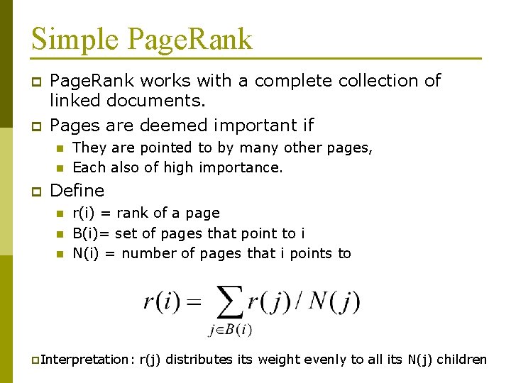
Simple Page. Rank p p Page. Rank works with a complete collection of linked documents. Pages are deemed important if n n p They are pointed to by many other pages, Each also of high importance. Define n n n r(i) = rank of a page B(i)= set of pages that point to i N(i) = number of pages that i points to p. Interpretation: r(j) distributes its weight evenly to all its N(j) children

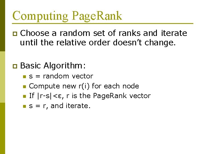
Computing Page. Rank p Choose a random set of ranks and iterate until the relative order doesn’t change. p Basic Algorithm: n n s = random vector Compute new r(i) for each node If |r-s|<ε, r is the Page. Rank vector s = r, and iterate.

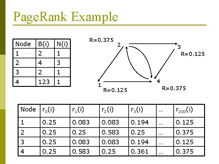
Page. Rank Example Node B(i) N(i) 1 2 4 3 3 2 1 4 123 1 R=0. 375 1 2 3 R=0. 125 4 R=0. 375 R=0. 125 Node r 0(i) r 1(i) r 2(i) r 3(i) … r 200(i) 1 0. 25 0. 083 0. 194 … 0. 125 2 0. 25 0. 583 0. 25 … 0. 375 3 0. 25 0. 083 0. 194 … 0. 125 4 0. 25 0. 583 0. 25 0. 361 … 0. 375

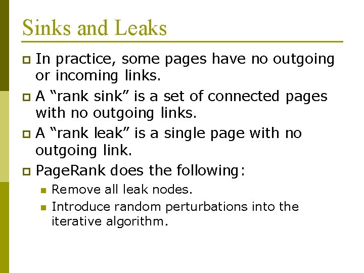
Sinks and Leaks In practice, some pages have no outgoing or incoming links. p A “rank sink” is a set of connected pages with no outgoing links. p A “rank leak” is a single page with no outgoing link. p Page. Rank does the following: p n n Remove all leak nodes. Introduce random perturbations into the iterative algorithm.

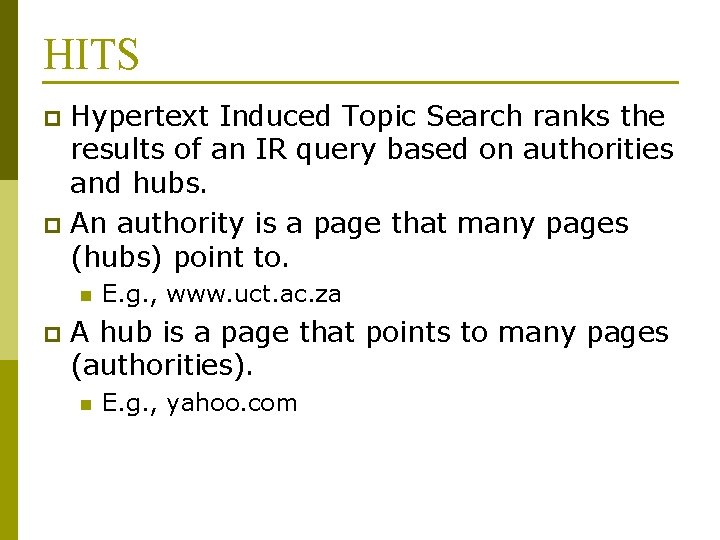
HITS Hypertext Induced Topic Search ranks the results of an IR query based on authorities and hubs. p An authority is a page that many pages (hubs) point to. p n p E. g. , www. uct. ac. za A hub is a page that points to many pages (authorities). n E. g. , yahoo. com

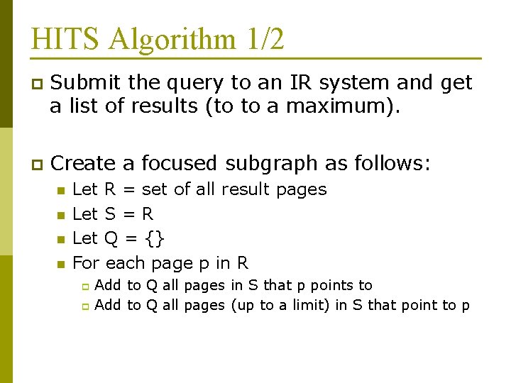
HITS Algorithm 1/2 p Submit the query to an IR system and get a list of results (to to a maximum). p Create a focused subgraph as follows: n n Let R = set of all result pages Let S = R Let Q = {} For each page p in R Add to Q all pages in S that p points to p Add to Q all pages (up to a limit) in S that point to p p

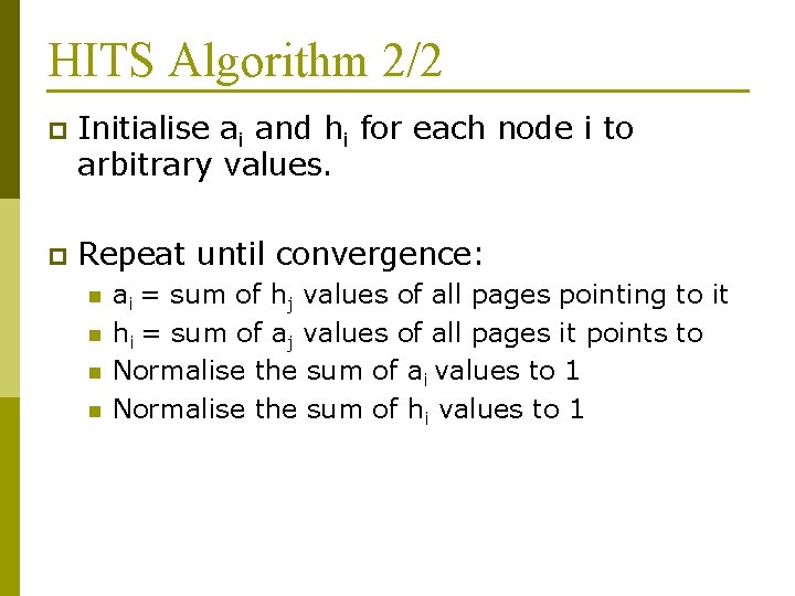
HITS Algorithm 2/2 p Initialise ai and hi for each node i to arbitrary values. p Repeat until convergence: n n ai = sum of hj values of all pages pointing to it hi = sum of aj values of all pages it points to Normalise the sum of ai values to 1 Normalise the sum of hi values to 1

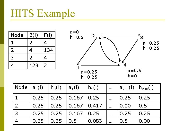
HITS Example Node B(i) F(i) 1 2 4 134 3 2 4 4 123 2 a=0 h=0. 5 1 2 3 a=0. 25 h=0. 25 4 a=0. 5 h=0 a=0. 25 h=0. 25 Node a 0(i) h 0(i) a 1(i) h 1(i) … a 200(i) h 200(i) 1 0. 25 0. 167 0. 25 … 0. 25 2 0. 25 0. 167 0. 417 … 0. 00 0. 5 3 0. 25 0. 167 0. 25 … 0. 25 4 0. 25 0. 083 … 0. 5 0. 00

References p p p Arasu, A. , J. Cho, H. Garcia-Molina, A. Paepcke and S. Raghavan (2001). “Searching the Web”, ACM Transactions on Internet Technology, Vol 1. , No. 1, August 2001, pp. 243. Bell, T. C. , J. G. Cleary and I. H. Witten (1990) Text Compression, Prentice Hall, New Jersey. Berry, M. W. and M. Browne (1999) Understanding Search Engines: Mathematical Modelling and Text Retrieval, SIAM, Philadelphia. Deerwester, S. T. Dumais, T. K. Landauer, G. W. Furnas and R. A. Harshman (1990). - no figures, “Indexing by latent semantic analysis”, Journal of the Society for Information Science, Vol. 41, No. 6, pp. 391 -407. Witten, I. H. , A. Moffat and T. C. Bell (1999) Managing Gigabytes, Morgan Kauffman, San Francisco.