Information Bottleneck versus Maximum Likelihood Felix Polyakov A

Information Bottleneck versus Maximum Likelihood Felix Polyakov

A simple example. . . A coin is known to be biased The coin is tossed three times – two heads and one tail Use ML to estimate the probability of throwing a head −p(head) = P −p(tail) = 1 - P ØTry P = 0. 2 L(O) = 0. 2 * 0. 8 = 0. 032 ØTry P = 0. 4 L(O) = 0. 4 * 0. 6 = 0. 096 ØTry P = 0. 6 L(O) = 0. 6 * 0. 4 = 0. 144 ØTry P = 0. 8 L(O) = 0. 8 * 0. 2 = 0. 128 Likelihood of the Data • Model: Probability of a head

A bit more complicated example… : Mixture Model • Three baskets with white (O = 1), grey (O = 2), and black (O = 3) balls • B 1 B 2 B 3 15 balls were drawn as follows: 1. Choose a basket according to p(i) = bi 2. Draw the ball j from basket i with probability • Use ML to estimate given the observations: sequence of balls’ colors

• Likelihood of observations • Log Likelihood of observations • Maximal Likelihood of observations
![Likelihood of the observed data x – hidden random variables [e. g. basket] y](http://slidetodoc.com/presentation_image/f721e997218f6b118bf331aad28f06aa/image-5.jpg "Likelihood of the observed data x – hidden random variables [e. g. basket] y")
Likelihood of the observed data x – hidden random variables [e. g. basket] y – observed random variables [e. g. color] - model parameters [e. g. they define p(y|x)] 0 – current estimate of model parameters
 1. Expectation − Compute − Get 2. Maximization − • •")
Expectation-maximization algorithm (I) 1. Expectation − Compute − Get 2. Maximization − • • EM algorithm converges to local maxima

Log-likelihood is non-decreasing, examples

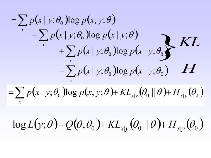
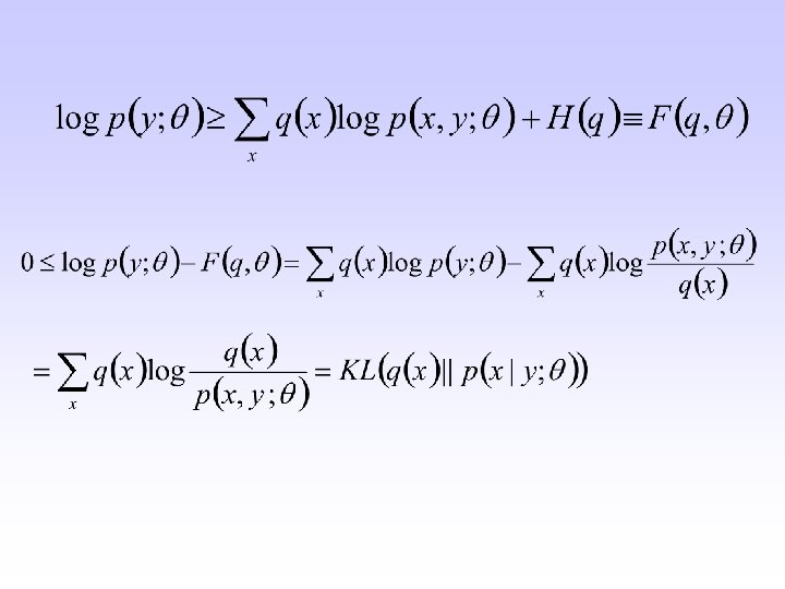
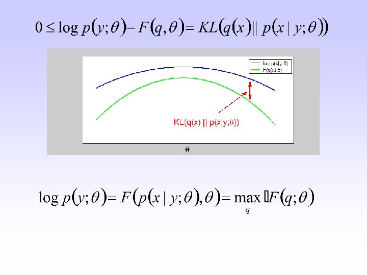
EM – another approach Ø Goal: Jensen’s inequality for concave function
 1. Expectation 2. Maximization (I) and (II) are equivalent")
Expectation-maximization algorithm (II) 1. Expectation 2. Maximization (I) and (II) are equivalent

Scheme of the approach
- Slides: 13