INFO 2950 Prof Carla Gomes gomescs cornell edu

INFO 2950 Prof. Carla Gomes gomes@cs. cornell. edu Module Algorithms and Growth Rates Rose, Chapter 3 1

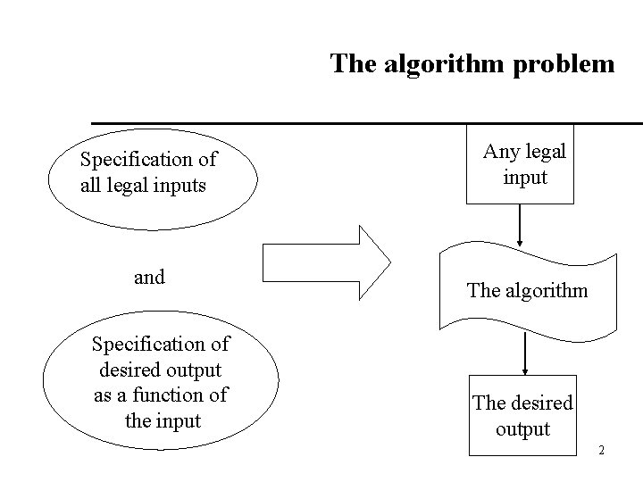
The algorithm problem Specification of all legal inputs and Specification of desired output as a function of the input Any legal input The algorithm The desired output 2

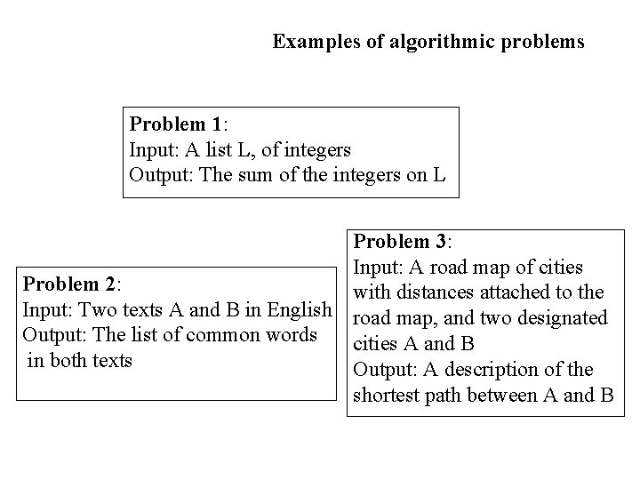
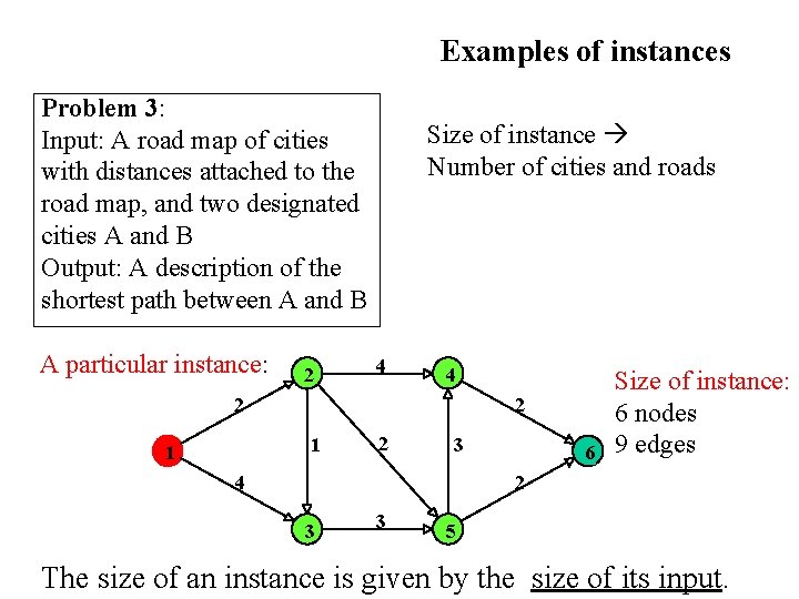
Examples of algorithmic problems Problem 1: Input: A list L, of integers Output: The sum of the integers on L Problem 3: Input: A road map of cities Problem 2: with distances attached to the Input: Two texts A and B in English road map, and two designated Output: The list of common words cities A and B in both texts Output: A description of the shortest path between A and B

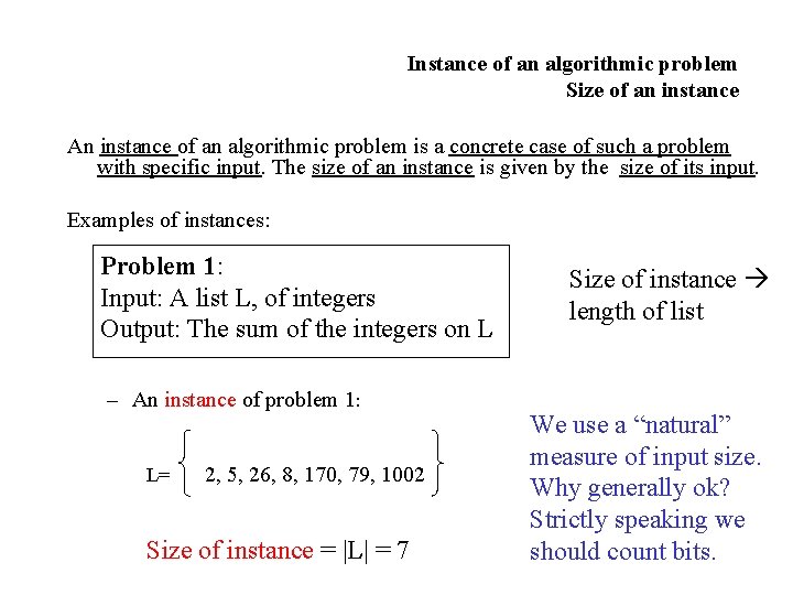
Instance of an algorithmic problem Size of an instance An instance of an algorithmic problem is a concrete case of such a problem with specific input. The size of an instance is given by the size of its input. Examples of instances: Problem 1: Input: A list L, of integers Output: The sum of the integers on L – An instance of problem 1: L= 2, 5, 26, 8, 170, 79, 1002 Size of instance = |L| = 7 Size of instance length of list We use a “natural” measure of input size. Why generally ok? Strictly speaking we should count bits.

Examples of instances Problem 3: Input: A road map of cities with distances attached to the road map, and two designated cities A and B Output: A description of the shortest path between A and B A particular instance: 2 Size of instance Number of cities and roads 4 4 2 2 1 1 2 3 4 6 Size of instance: 6 nodes 9 edges 2 3 3 5 The size of an instance is given by the size of its input.

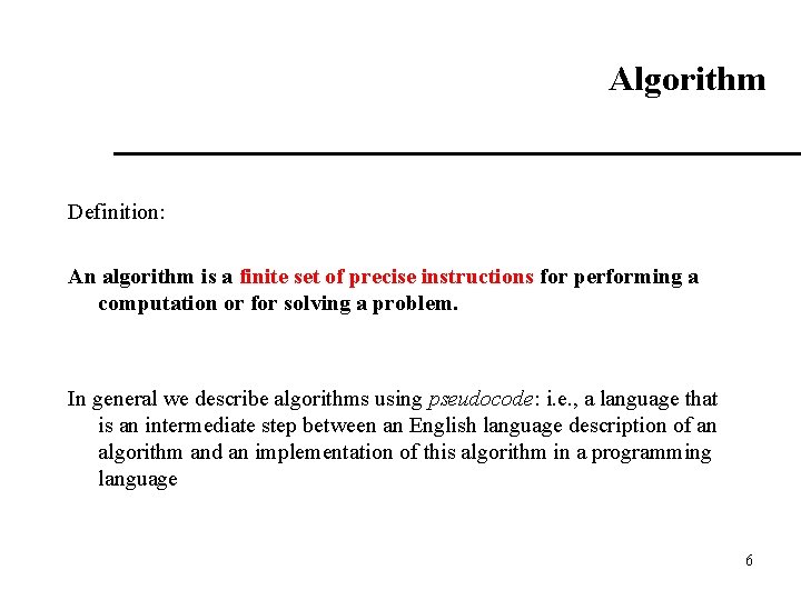
Algorithm Definition: An algorithm is a finite set of precise instructions for performing a computation or for solving a problem. In general we describe algorithms using pseudocode: i. e. , a language that is an intermediate step between an English language description of an algorithm and an implementation of this algorithm in a programming language 6

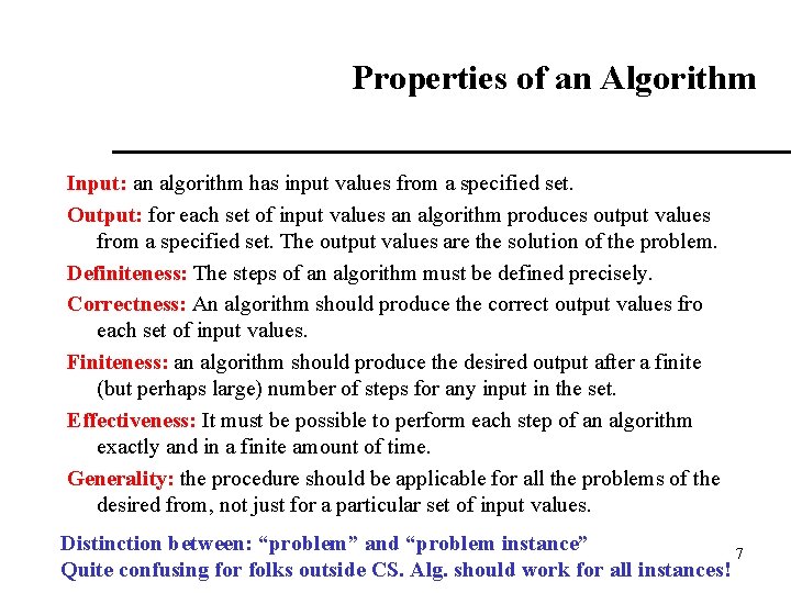
Properties of an Algorithm Input: an algorithm has input values from a specified set. Output: for each set of input values an algorithm produces output values from a specified set. The output values are the solution of the problem. Definiteness: The steps of an algorithm must be defined precisely. Correctness: An algorithm should produce the correct output values fro each set of input values. Finiteness: an algorithm should produce the desired output after a finite (but perhaps large) number of steps for any input in the set. Effectiveness: It must be possible to perform each step of an algorithm exactly and in a finite amount of time. Generality: the procedure should be applicable for all the problems of the desired from, not just for a particular set of input values. Distinction between: “problem” and “problem instance” 7 Quite confusing for folks outside CS. Alg. should work for all instances!

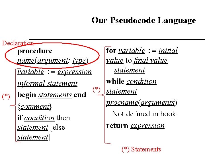
Our Pseudocode Language Declaration procedure name(argument: type) variable : = expression informal statement (*) begin statements end {comment} if condition then statement [else statement] for variable : = initial value to final value statement while condition statement procname(arguments) Not defined in book: return expression (*) Statements

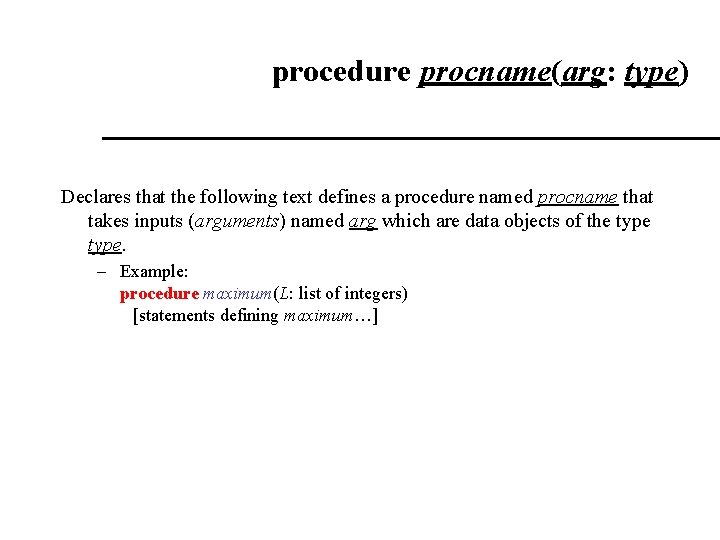
procedure procname(arg: type) Declares that the following text defines a procedure named procname that takes inputs (arguments) named arg which are data objects of the type. – Example: procedure maximum(L: list of integers) [statements defining maximum…]

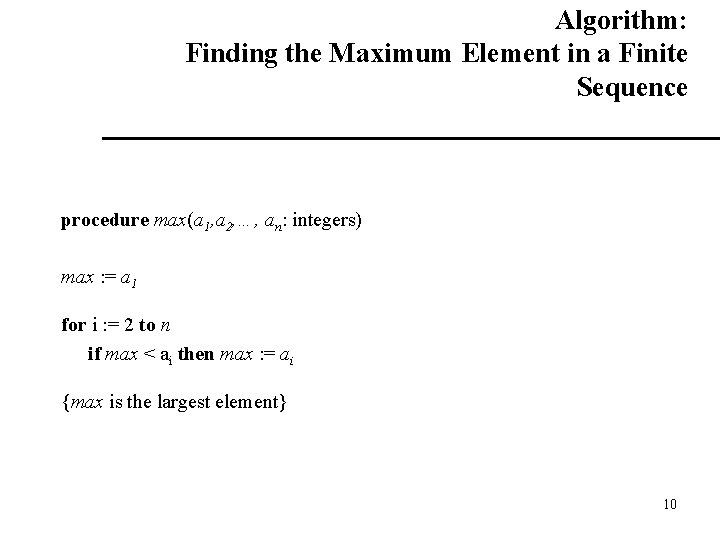
Algorithm: Finding the Maximum Element in a Finite Sequence procedure max(a 1, a 2, …, an: integers) max : = a 1 for i : = 2 to n if max < ai then max : = ai {max is the largest element} 10

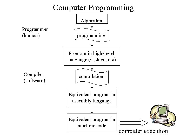
Computer Programming Algorithm Programmer (human) programming Program in high-level language (C, Java, etc) Compiler (software) compilation Equivalent program in assembly language Equivalent program in machine code computer execution

Searching Algorithms Searching problems: the problem of locating an element in an ordered list. Example: searching for a word in a dictionary. 12

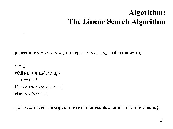
Algorithm: The Linear Search Algorithm procedure linear search( x: integer, a 1, a 2, …, an: distinct integers) i : = 1 while (i ≤ n and x ai ) i : = i +1 if i < n then location : = i else location : = 0 {location is the subscript of the term that equals x, or is 0 if x is not found} 13

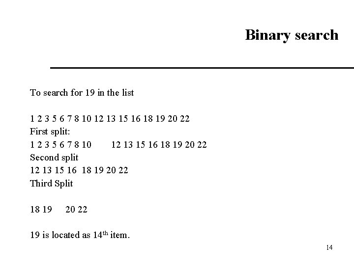
Binary search To search for 19 in the list 1 2 3 5 6 7 8 10 12 13 15 16 18 19 20 22 First split: 1 2 3 5 6 7 8 10 12 13 15 16 18 19 20 22 Second split 12 13 15 16 18 19 20 22 Third Split 18 19 20 22 19 is located as 14 th item. 14

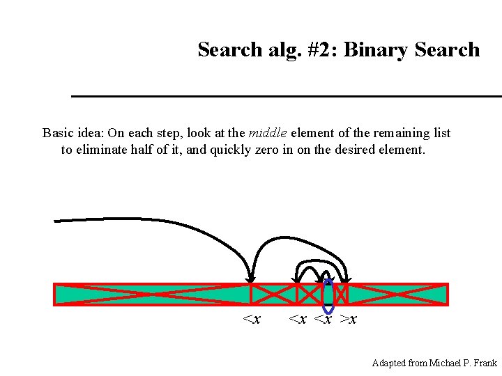
Search alg. #2: Binary Search Basic idea: On each step, look at the middle element of the remaining list to eliminate half of it, and quickly zero in on the desired element. <x <x <x >x Adapted from Michael P. Frank

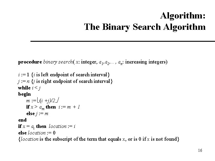
Algorithm: The Binary Search Algorithm procedure binary search( x: integer, a 1, a 2, …, an: increasing integers) i : = 1 {i is left endpoint of search interval} j : = n {j is right endpoint of search interval} while i < j begin m : = (i +j)/2 if x > am then i : = m + 1 else j : = m end if x = ai then location : = i else location : = 0 {location is the subscript of the term that equals x, or is 0 if x is not found} 16

Just because we know how to solve a given problem – we have an algorithm - that does not mean that the problem can be solved. The procedure (algorithm) may be so inefficient that it would not be possible to solve the problem within a useful period of time. So we would like to have an idea in terms of the “complexity” of our algorithm. 17

Complexity of Algorithms 18

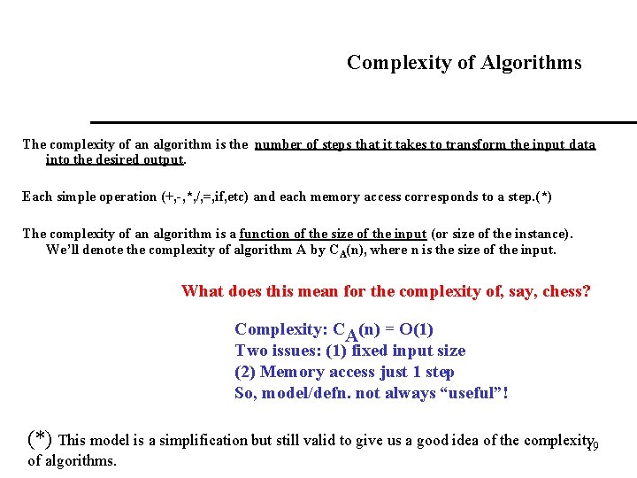
Complexity of Algorithms The complexity of an algorithm is the number of steps that it takes to transform the input data into the desired output. Each simple operation (+, -, *, /, =, if, etc) and each memory access corresponds to a step. (*) The complexity of an algorithm is a function of the size of the input (or size of the instance). We’ll denote the complexity of algorithm A by CA(n), where n is the size of the input. What does this mean for the complexity of, say, chess? Complexity: CA(n) = O(1) Two issues: (1) fixed input size (2) Memory access just 1 step So, model/defn. not always “useful”! (*) This model is a simplification but still valid to give us a good idea of the complexity 19 of algorithms.

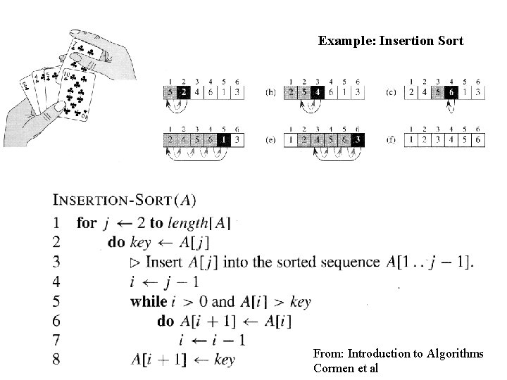
Example: Insertion Sort From: Introduction to Algorithms 20 Cormen et al

Different notions of complexity Worst case complexity of an algorithm A – the maximum number of computational steps required for the execution of Algorithm A, over all the inputs of the same size, s. It provides an upper bound for an algorithm. The worst that can happen given the most difficult instance – the pessimistic view. Best case complexity of an algorithm A the minimum number of computational steps required for the execution of Algorithm A, over all the inputs of the same size, s. The most optimistic view of an algorithm– it tells us the least work a particular algorithm could possibly get away with for some one input of a fixed size – we have the chance to pick the easiest input of a given size. Linear search: Worst cost? Best cost? Average cost? 21

Average case complexity of an algorithm A - i. e. , the average amount of resources the algorithm consumes assuming some plausible frequency of occurrence of each input. Figuring out the average cost is much more difficult than figuring out either the worst-cost or best-cost e. g. , we have to assume a given probability distribution for the types of inputs we get. P ractical difficulty: What is the distribution of “real-world” problem instances? 22

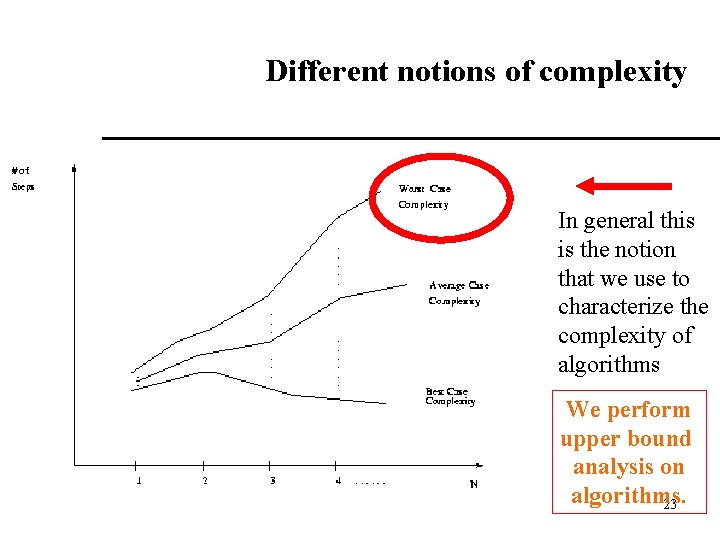
Different notions of complexity In general this is the notion that we use to characterize the complexity of algorithms We perform upper bound analysis on algorithms. 23

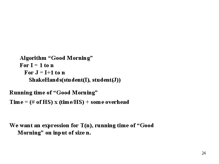
Algorithm “Good Morning” For I = 1 to n For J = I+1 to n Shake. Hands(student(I), student(J)) Running time of “Good Morning” Time = (# of HS) x (time/HS) + some overhead We want an expression for T(n), running time of “Good Morning” on input of size n. 24

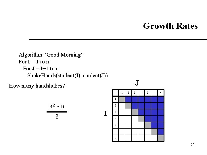
Growth Rates Algorithm “Good Morning” For I = 1 to n For J = I+1 to n Shake. Hands(student(I), student(J)) J How many handshakes? 1 2 3 4 5 n 1 n 2 - n 2 2 I 3 4 5 n 25

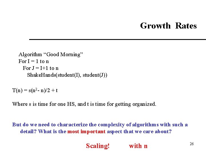
Growth Rates Algorithm “Good Morning” For I = 1 to n For J = I+1 to n Shake. Hands(student(I), student(J)) T(n) = s(n 2 - n)/2 + t Where s is time for one HS, and t is time for getting organized. But do we need to characterize the complexity of algorithms with such a detail? What is the most important aspect that we care about? Scaling! with n 26

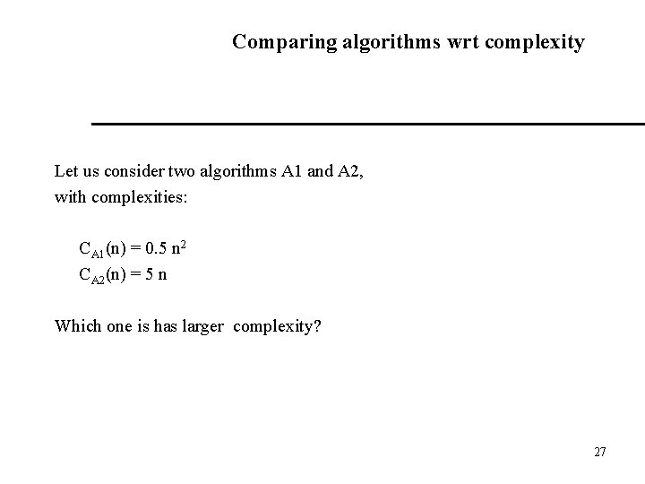
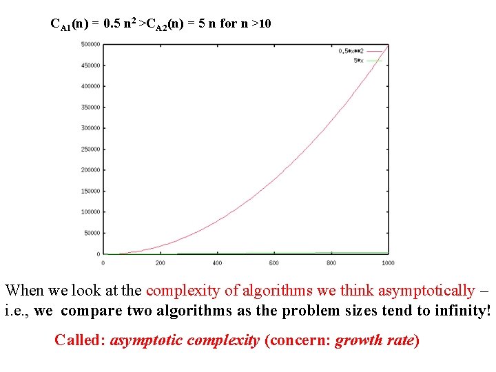
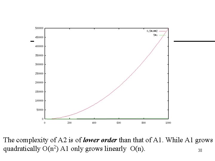
Comparing algorithms wrt complexity Let us consider two algorithms A 1 and A 2, with complexities: CA 1(n) = 0. 5 n 2 CA 2(n) = 5 n Which one is has larger complexity? 27

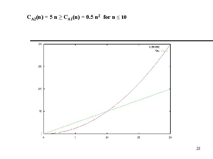
CA 2(n) = 5 n ≥ CA 1(n) = 0. 5 n 2 for n ≤ 10 28

CA 1(n) = 0. 5 n 2 >CA 2(n) = 5 n for n >10 When we look at the complexity of algorithms we think asymptotically – i. e. , we compare two algorithms as the problem sizes tend to infinity! Called: asymptotic complexity (concern: growth rate)

Game I’m thinking of an integer between [1, 64]. You guess the number. To your guesses my answer is, High, Low, Yes. How many guesses do you need in the worst case? What strategy are we assuming? 30

Growth Rates In general we only worry about growth rates because: Our main objective is to analyze the cost performance of algorithms asymptotically. (reasonable in part because computers get faster and faster every year. ) Another obstacle to having the exact cost of algorithms is that sometimes the algorithms are quite complicated to analyze. When analyzing an algorithm we are not that interested in the exact time the algorithm takes to run – often we only want to compare two algorithms for the same problem – the thing that makes one algorithm more desirable than another is its growth rate relative to the other algorithm’s growth rate. 31

Growth of Rates Algorithm analysis is concerned with: • Type of function that describes run time (we ignore constant factors since different machines have different speed/cycle) • Large values of n 32

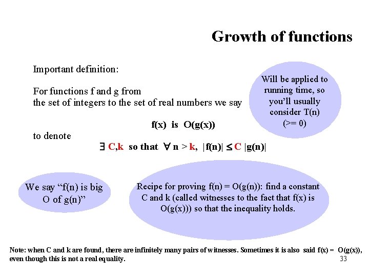
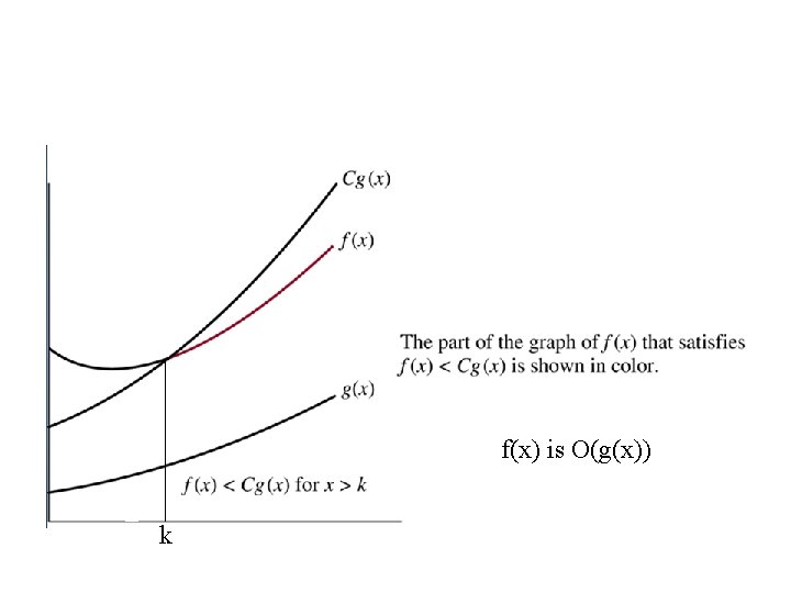
Growth of functions Important definition: For functions f and g from the set of integers to the set of real numbers we say to denote f(x) is O(g(x)) Will be applied to running time, so you’ll usually consider T(n) (>= 0) C, k so that n > k, |f(n)| C |g(n)| We say “f(n) is big O of g(n)” Recipe for proving f(n) = O(g(n)): find a constant C and k (called witnesses to the fact that f(x) is O(g(x))) so that the inequality holds. Note: when C and k are found, there are infinitely many pairs of witnesses. Sometimes it is also said f(x) = O(g(x)), even though this is not a real equality. 33

f(x) is O(g(x)) k

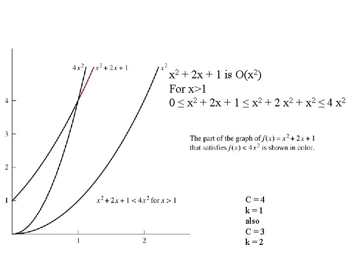
x 2 + 2 x + 1 is O(x 2) For x>1 0 ≤ x 2 + 2 x + 1 ≤ x 2 + 2 x 2 + x 2 ≤ 4 x 2 C = 4 k = 1 also C = 3 k = 2

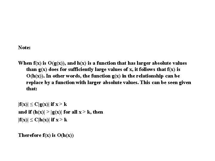
Note: When f(x) is O(g(x)), and h(x) is a function that has larger absolute values than g(x) does for sufficiently large values of x, it follows that f(x) is O(h(x)). In other words, the function g(x) in the relationship can be replace by a function with larger absolute values. This can be seen given that: |f(x)| ≤ C|g(x)| if x > k and if (h(x)| > |g(x)| for all x > k, then |f(x)| ≤ C|h(x)| if x > k Therefore f(x) is O(h(x))

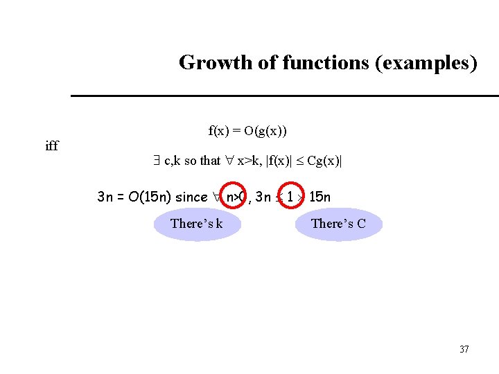
Growth of functions (examples) iff f(x) = O(g(x)) c, k so that x>k, |f(x)| Cg(x)| 3 n = O(15 n) since n>0, 3 n 1 15 n There’s k There’s C 37

The complexity of A 2 is of lower order than that of A 1. While A 1 grows quadratically O(n 2) A 1 only grows linearly O(n). 38

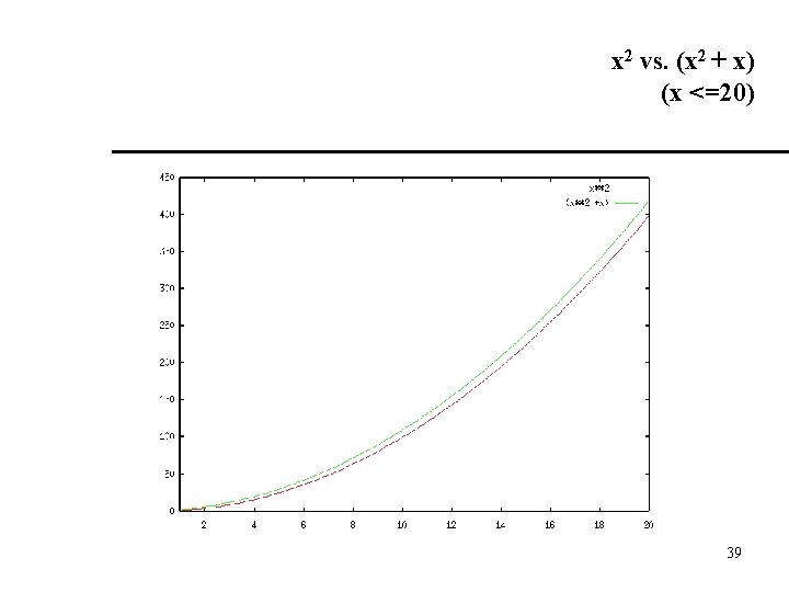
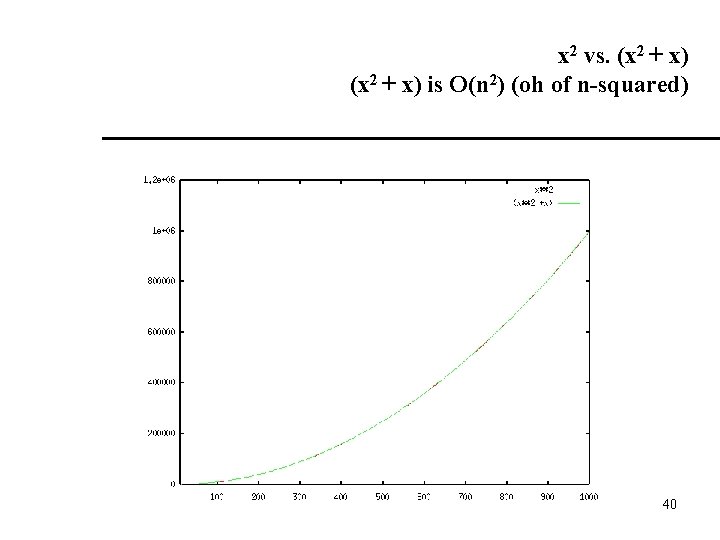
x 2 vs. (x 2 + x) (x <=20) 39

x 2 vs. (x 2 + x) is O(n 2) (oh of n-squared) 40

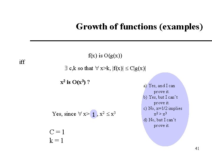
Growth of functions (examples) iff f(x) is O(g(x)) c, k so that x>k, |f(x)| C|g(x)| x 2 is O(x 3) ? 2 x 3 Yes, since x> __, x 1 a) Yes, and I can prove it. b) Yes, but I can’t prove it. c) No, x=1/2 implies x 2 > x 3 d) No, but I can’t prove it. C = 1 k = 1 41

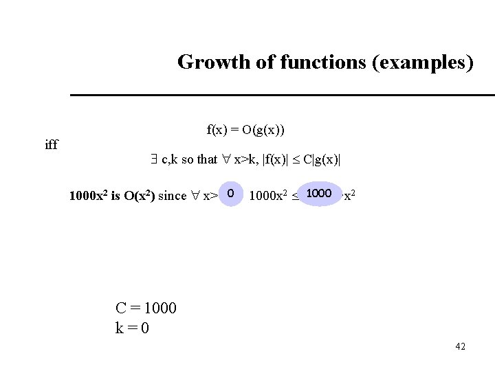
Growth of functions (examples) iff f(x) = O(g(x)) c, k so that x>k, |f(x)| C|g(x)| 2 ____ ·x 2 0 1000 x 2 is O(x 2) since x> __, 1000 x C = 1000 k = 0 42

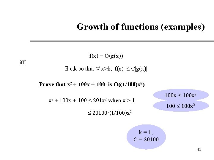
Growth of functions (examples) iff f(x) = O(g(x)) c, k so that x>k, |f(x)| C|g(x)| Prove that x 2 + 100 x + 100 is O((1/100)x 2) x 2 + 100 x + 100 201 x 2 when x > 1 20100·(1/100)x 2 100 x 2 100 x 2 k = 1, C = 20100 43

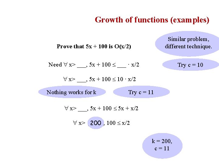
Growth of functions (examples) Similar problem, different technique. Prove that 5 x + 100 is O(x/2) Need x> ___, 5 x + 100 ___ · x/2 Try c = 10 x> ___, 5 x + 100 10 · x/2 Nothing works for k Try c = 11 x> ___, 5 x + 100 5 x + x/2 x> __ _, 100 x/2 200 k = 200, c = 11

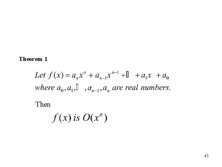
Theorem 1 Then 45

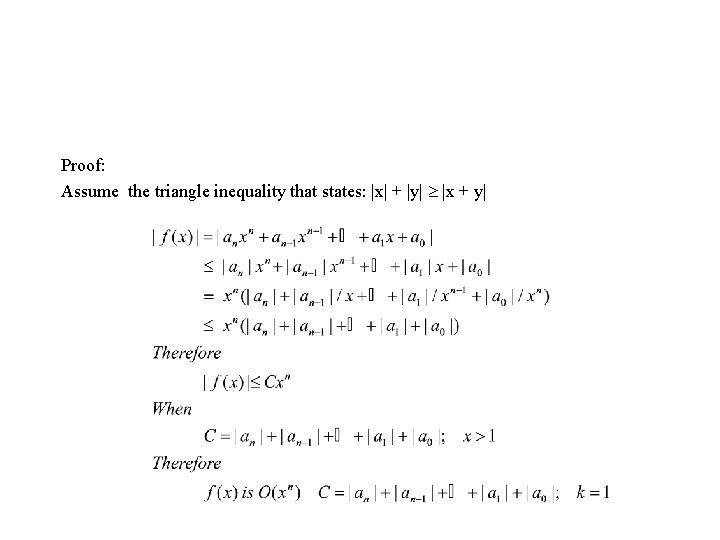
Proof: Assume the triangle inequality that states: |x| + |y| |x + y|

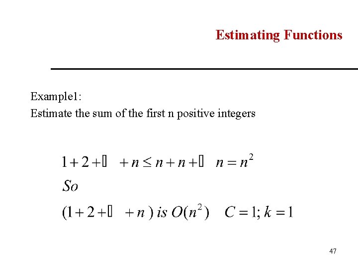
Estimating Functions Example 1: Estimate the sum of the first n positive integers 47

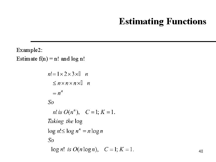
Estimating Functions Example 2: Estimate f(n) = n! and log n! 48

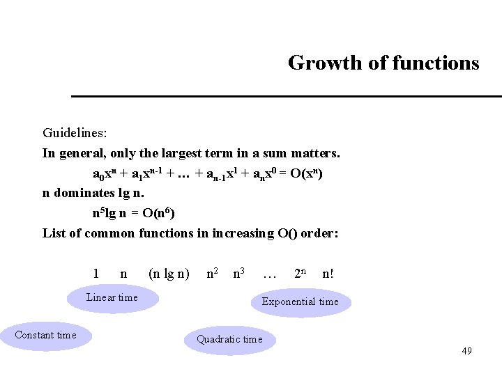
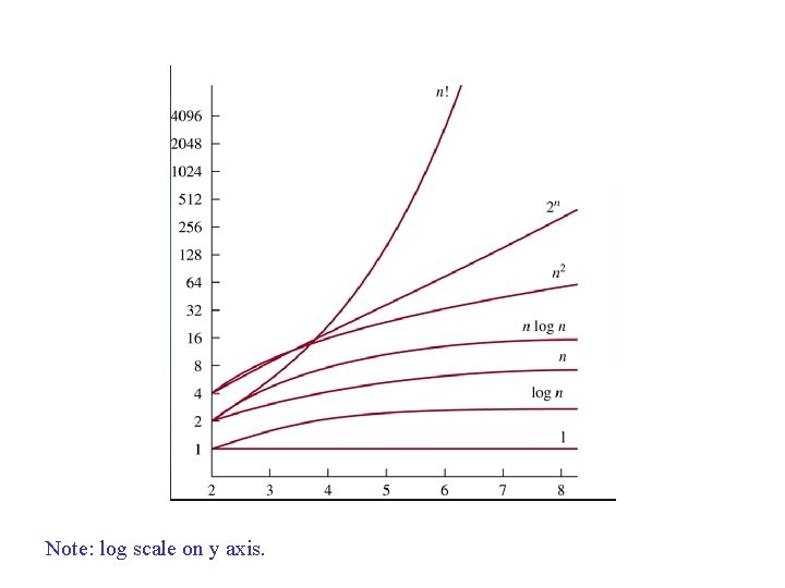
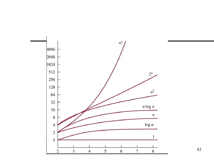
Growth of functions Guidelines: In general, only the largest term in a sum matters. a 0 xn + a 1 xn-1 + … + an-1 x 1 + anx 0 = O(xn) n dominates lg n. n 5 lg n = O(n 6) List of common functions in increasing O() order: 1 n (n lg n) n 2 n 3 … 2 n n! Linear time Constant time Exponential time Quadratic time 49

Note: log scale on y axis.

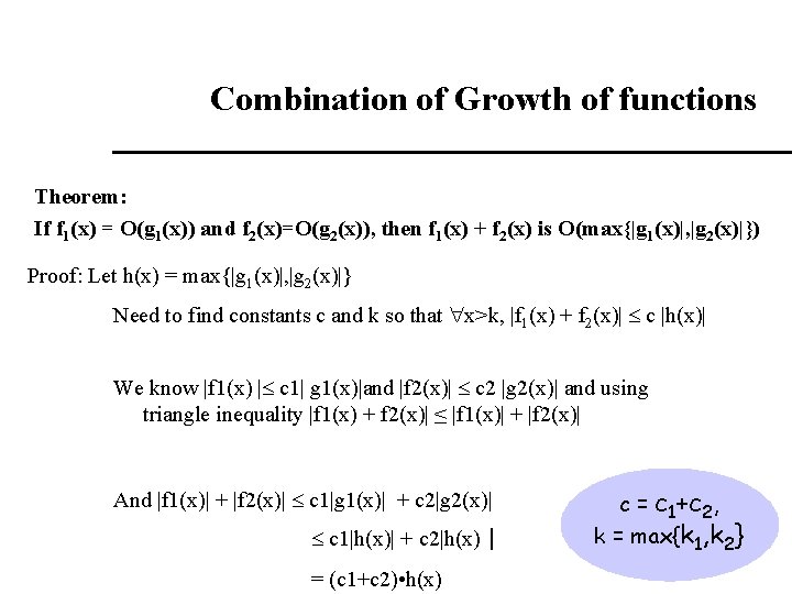
Combination of Growth of functions Theorem: If f 1(x) = O(g 1(x)) and f 2(x)=O(g 2(x)), then f 1(x) + f 2(x) is O(max{|g 1(x)|, |g 2(x)|}) Proof: Let h(x) = max{|g 1(x)|, |g 2(x)|} Need to find constants c and k so that x>k, |f 1(x) + f 2(x)| c |h(x)| We know |f 1(x) | c 1| g 1(x)|and |f 2(x)| c 2 |g 2(x)| and using triangle inequality |f 1(x) + f 2(x)| ≤ |f 1(x)| + |f 2(x)| And |f 1(x)| + |f 2(x)| c 1|g 1(x)| + c 2|g 2(x)| c 1|h(x)| + c 2|h(x) | = (c 1+c 2) • h(x) c = c 1+c 2, k = max{k 1, k 2} 51

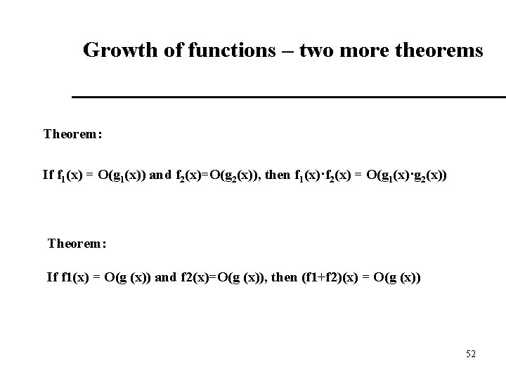
Growth of functions – two more theorems Theorem: If f 1(x) = O(g 1(x)) and f 2(x)=O(g 2(x)), then f 1(x)·f 2(x) = O(g 1(x)·g 2(x)) Theorem: If f 1(x) = O(g (x)) and f 2(x)=O(g (x)), then (f 1+f 2)(x) = O(g (x)) 52

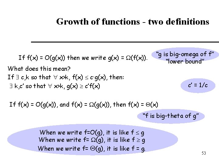
Growth of functions - two definitions If f(x) = O(g(x)) then we write g(x) = (f(x)). What does this mean? If c, k so that x>k, f(x) c·g(x), then: k, c’ so that x>k, g(x) c’f(x) “g is big-omega of f” “lower bound” c’ = 1/c If f(x) = O(g(x)), and f(x) = (g(x)), then f(x) = (x) “f is big-theta of g” When we write f=O(g), it is like f g When we write f= (g), it is like f = g. 53

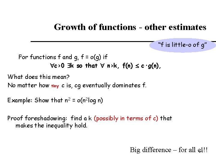
Growth of functions - other estimates “f is little-o of g” For functions f and g, f = o(g) if c>0 k so that n>k, f(n) c·g(n), What does this mean? No matter how tiny c is, cg eventually dominates f. Example: Show that n 2 = o(n 2 log n) Proof foreshadowing: find a k (possibly in terms of c) that makes the inequality hold. Big difference – for all c!!! 54

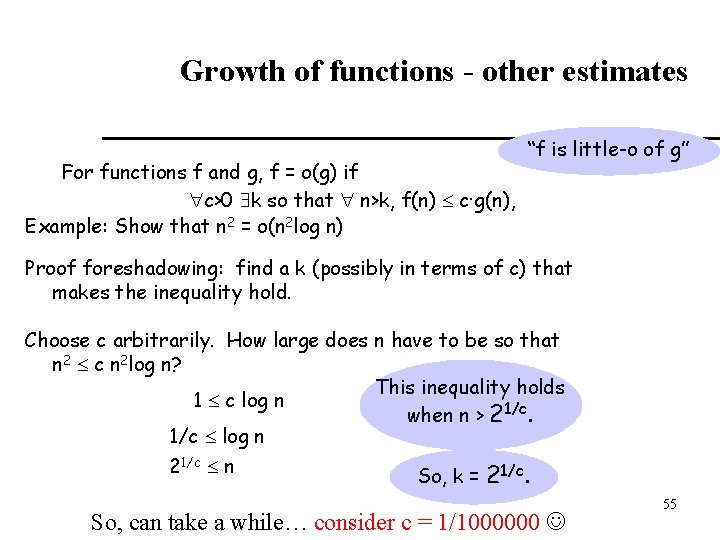
Growth of functions - other estimates For functions f and g, f = o(g) if c>0 k so that n>k, f(n) c·g(n), Example: Show that n 2 = o(n 2 log n) “f is little-o of g” Proof foreshadowing: find a k (possibly in terms of c) that makes the inequality hold. Choose c arbitrarily. How large does n have to be so that n 2 c n 2 log n? This inequality holds 1 c log n when n > 21/c. 1/c log n 21/c n So, k = 21/c. So, can take a while… consider c = 1/1000000 55

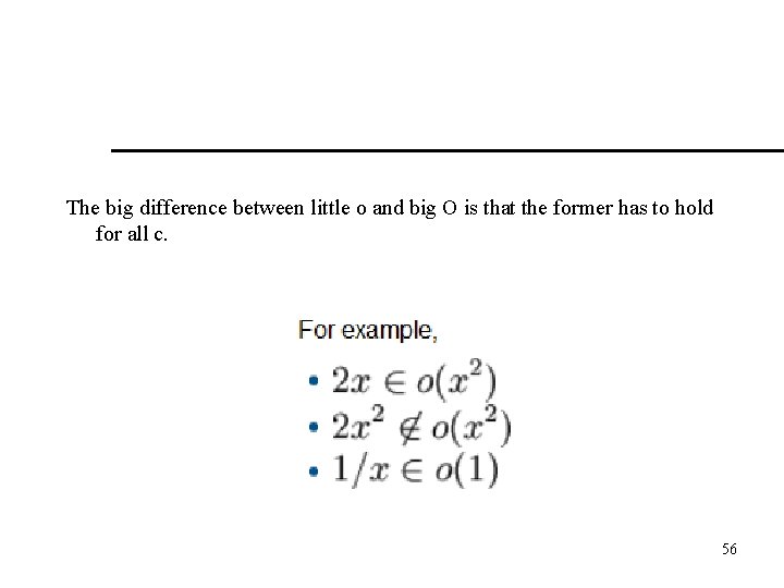
The big difference between little o and big O is that the former has to hold for all c. 56

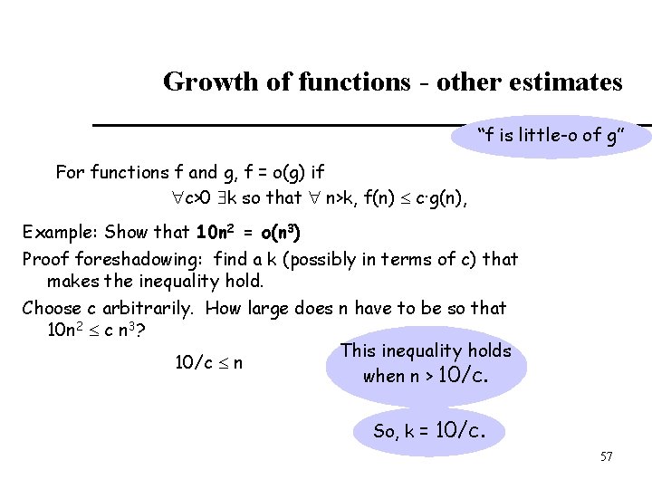
Growth of functions - other estimates “f is little-o of g” For functions f and g, f = o(g) if c>0 k so that n>k, f(n) c·g(n), Example: Show that 10 n 2 = o(n 3) Proof foreshadowing: find a k (possibly in terms of c) that makes the inequality hold. Choose c arbitrarily. How large does n have to be so that 10 n 2 c n 3? This inequality holds 10/c n when n > 10/c. So, k = 10/c. 57

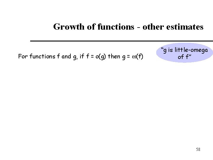
Growth of functions - other estimates For functions f and g, if f = o(g) then g = (f) “g is little-omega of f” 58

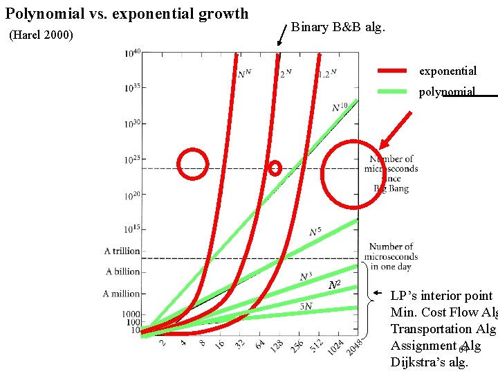
How do computer scientists differentiate between good (efficient) and bad (not efficient) algorithms? 60

How do computer scientists differentiate between good (efficient) and bad (not efficient) algorithms? The yardstick is that any algorithm that runs in no more than polynomial time is an efficient algorithm; everything else is not. 61

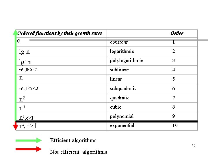
Ordered functions by their growth rates c Order constant 1 lg n lgc n logarithmic 2 polylogarithmic 3 nr , 0<r<1 sublinear 4 n linear 5 nr , 1<r<2 subquadratic 6 n 2 n 3 nc, c≥ 1 rn, r>1 quadratic 7 cubic 8 polynomial 9 exponential 10 Efficient algorithms 62 Not efficient algorithms

63

Polynomial vs. exponential growth (Harel 2000) Binary B&B alg. exponential polynomial N 2 LP’s interior point Min. Cost Flow Alg Transportation Alg Assignment Alg 64 Dijkstra’s alg.