INFLATION AND THE MULTIVERSE Alex Vilenkin Tufts Institute

INFLATION AND THE MULTIVERSE Alex Vilenkin Tufts Institute of Cosmology Prague, Sept. 2018

The multiverse picture that has emerged from inflationary cosmology. Remote regions beyond our horizon are strikingly different from what we observe here. Review of inflation Multiverse scenario How can we test this?

Inflation – fast, accelerated expansion in the early universe • During inflation: V “Slow roll” • Negative pressure (tension): Our vacuum scalar field (inflaton) V

Inflation – fast, accelerated expansion in the early universe • During inflation: V “Slow roll” • Negative pressure (tension): scalar field (inflaton) Our vacuum • Accelerated expansion: (repulsive gravity) – scale factor. • Horizon distance: . V

Inflationary scenario Guth (1981); Linde (1982) • Start with a high-energy field region of size R > H-1. “Big bang” time Inflation • It expands by a huge factor. • Field energy thermalizes into hot plasma. Explains some puzzling features of the big bang. Large-scale homogeneity and flatness. Small density perturbations. Mukhanov & Chibisov (1981)

Conditions for inflation “Slow roll” Slow roll: Our vacuum

Conditions for inflation “Slow roll” Slow roll: Our vacuum Conditions for slow roll: – Planck mass Planck units:

Amount of inflation “Slow roll” Amount of inflation: Number of e-folds: We need .

Variety of models Energy Density false vacuum “Slow roll” Scalar Field Models with multiple scalar fields. Focus on this Some of the predictions are robust & confirmed by the data: Flat large-scale geometry (at ~1% accuracy). Nearly scale-invariant spectrum of adiabatic, Gaussian density perturbations. WMAP, Planck, Galaxy surveys

Beyond the horizon: eternal inflation

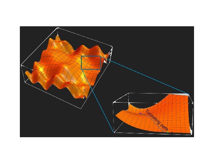
Energy Density In models where false vacuum decays through quantum tunneling: false vacuum “Slow roll” Scalar Field You are here False vacuum “Bubble universes” Inflation is eternal

Spacetime of a bubble universe t A moment of time Big bang Bubble wall Nucleation x We cannot travel to other bubbles. Viewed from inside, each bubble is an infinite universe.

Particle theories with extra dimensions (including string theory) predict a vast landscape of vacua with diverse properties. Bousso & Polchinski (2000) Susskind (2003) Bubbles of all types will be produced in the course of eternal inflation. The multiverse

How can we test multiverse models?

How can we test multiverse models? Bubble collisions can leave an imprint on the CMB (round hot spots). This would be a direct test of eternal inflation. Chang, Kleban & Levi (2008) Polarization signal. Feeney, Johnson, Mortlock & Peiris (2010) Czech et. al. (2011) The search is now on…

How can we test multiverse models? Bubble collisions can leave an imprint on the CMB (round hot spots). This would be a direct test of eternal inflation. Chang, Kleban & Levi (2008) Polarization signal. Feeney, Johnson, Mortlock & Peiris (2010) Czech et. al. (2011) The search is now on… Indirect tests: Predicting the values of the constants of Nature

Constants of Nature: Electron mass 0. 00511 Higgs mass 125 Neutrino mass < 10 -9 Planck mass 1019 Cosmological constant 10 -46 Appear to be fine-tuned for our existence. (in Ge. V)

Anthropic principle: We can live only in bio-friendly bubbles. This explains the fine-tuning. We can try to turn this into testable (statistical) predictions.

Anthropic principle: We can live only in bio-friendly bubbles. This explains the fine-tuning. We can try to turn this into testable (statistical) predictions. Strategy: Find the probability distribution P(X) for the values of some parameter X measured by a randomly picked observer. P(X) Make a prediction for a range of X at a specified confidence level. This assumes we are typical observers: Principle of mediocrity. X

The cosmological constant Energy density of our vacuum From particle physics: Riess et. al. (1998) Perlmutter et. al. (1998) Observation: Why is so small? – The cosmological constant problem. ? – The coincidence problem.

The cosmological constant Energy density of our vacuum From particle physics: Riess et. al. (1998) Perlmutter et. al. (1998) Observation: Why is so small? – The cosmological constant problem. ? – The coincidence problem. In the multiverse: (All other parameters are fixed. ) Anthropic range: Fraction of volume (from particle physics and theory of inflation). Number of observers per unit volume (in the range of interest). Weinberg (1987)

“Drake equation”: # of observers per star Number of stars per unit mass Not very sensitive to . Fraction of mass in large galaxies

“Drake equation”: # of observers per star Press & Schechter (1974) Number of stars per unit mass Not very sensitive to Fraction of mass in large galaxies . During the matter era: - . amplitude of density perturbations on galactic scale. At domination ( ), y ~ 1 means Q ~ 1 galaxies are formed. The distribution is peaked at y ~ 1. This is close to the present epoch.

Unnecessary fine-tuning Too few galaxies Weinberg (1987), A. V. (1995), Efstathiou (1995), Martel, Shapiro & Weinberg (1998) (Before measurement) 95% Explains the coincidence: is expected to dominate near the end of galaxy formation epoch. The agreement is better if extinctions by supernovae are taken into account. Totani et al. (2018) No alternative explanations. Our first evidence for the multiverse?

Unnecessary fine-tuning Too few galaxies Weinberg (1987), A. V. (1995), Efstathiou (1995), Martel, Shapiro & Weinberg (1998) (Before measurement) 95% Explains the coincidence: is expected to dominate near the end of galaxy formation epoch. The agreement is better if extinctions by supernovae are taken into account. Totani et al. (2018) No alternative explanations. Our first evidence for the multiverse? The distribution for Q, Ne , etc. depends on our model of the multiverse.

A GAUSSIAN MULTIVERSE

A simple model of landscape: a random Gaussian field Masoumi, A. V. & Yamada (2017, 2018) – N-dimensional field space. The landscape is characterized by the correlation function X e. g. , We shall assume (in Planck units).

A simple model of landscape: a random Gaussian field Masoumi, A. V. & Yamada (2017, 2018) – N-dimensional field space. The landscape is characterized by the correlation function X e. g. , We shall assume (in Planck units). Typical values: Slow roll conditions are strongly violated. Inflation can occur only in rare regions where V’ and V” are very small in some direction – most likely near saddle points (V’ = 0) or inflection points (V” = 0).

Single-field or multi-field inflation? Expand the potential near inflaton trajectory: Other fields X are dynamically important if Typical smallest mass: Yamada & A. V. (2018) Inflation is typically single-field. No isocurvature fluctuations. Negligible non-Gaussianity. .

Inflection point inflation Inflection point: V” = 0. Inflation range:

Inflection point inflation Inflection point: V” = 0. Inflation range: The number of e-folds: Probability distribution for Ne:

The distribution terms of correlators for Gaussian variables : , where can be expressed in . etc. , and similar for Probability of inflation with Ne e-folds: .

Distribution for the amplitude of density fluctuations: (over a wide range of values and falls off beyond that range) The distribution for the spectral index ns is also consistent with the data.

SUMMARY Inflation is a never ending process, with new “bubble universes” constantly being formed. Low-energy physics may be different in different bubbles. We can make statistical predictions. Successful prediction of . A simple model of sub-Planckian random Gaussian landscape is consistent with the present data.

BLACK HOLES FROM THE MULTIVERSE

As the inflaton field “rolls” towards our vacuum, it may tunnel to another vacuum. Our vacuum

Bubble nucleation Energy Density Coleman & De Luccia (1980) Bubbles of a lower-energy vacuum nucleate and expand during the slow roll: . Our Vacuum Scalar Field 1 Scalar Field 2

Bubble nucleation Time of nucleation t = tn: At t > tn : Scale-invariant size distribution: Nucleation rate

What happens to the bubbles when inflation ends? Matter • All bubbles are initially bigger than the horizon. • The bubble wall initially expands relativistically relative to matter. • It is quickly slowed down by particle scattering. • An expanding relativistic shell of matter is formed (a shock wave). • The bubble eventually comes within the horizon and collapses to a black hole. But there is more to the story…

What happens inside the bubble? Matter interior horizon • Bubbles of radius collapse to a singularity.

What happens inside the bubble? Matter interior horizon • Bubbles of radius collapse to a singularity. • If the bubble expands to a radius , its interior begins to inflate: But the universe outside the bubble is expanding much slower.

Inflating baby universe The “wormhole” is seen as a black hole by exterior observers. Exterior FRW region Black holes of mass have inflating baby universes inside.

Penrose diagram Shock Light propagates at 45 o. Future infinity • Some matter may follow the bubble into the wormhole. This changes the black hole mass. • Need numerical simulations to determine Mbh. .

Upper bound on BH mass • The affected region expands as . The universe outside of it is unperturbed. • The size of this region when it comes within the horizon is . • The largest BH that can fit into this region has mass

Global structure of spacetime • The baby universes will inflate eternally. • Bubbles of all possible vacua, including ours, will be formed.

The big picture Linde (1988) 46

Black hole mass Deng & A. V. (2018) M ~ Mmax (saturates the bound) Depending on microphysics, take a wide range of values. may

Mass distribution of black holes Fraction of dark matter density in black holes of mass ~ M : Use and .

Mass distribution of black holes Fraction of dark matter density in black holes of mass ~ M : Bubble nucleation rate . Minimal BH mass: . The mass distribution depends on 3 parameters: A discovery of black holes with the predicted distribution of masses would provide evidence for inflation – and for the multiverse. – mass within the horizon at teq.

Observational bounds 3 2 1 1 -Gamma-ray background from BH evaporation with 2 -CMB spectral distortions by accreting BH with .

Accounting for LIGO observations . BH merger rate observed by LIGO requires Note: BH produced by bubbles are non-rotating. for . . Sasaki et al (2016)

Supermassive black holes . • The largest BH we can expect to find in a galaxy has mass • Early formation of massive halos. • May have interesting signatures in CMB spectral distortions. Deng, A. V. & Yamada (2018) . .

Summary Vacuum bubbles may nucleate during inflation, leading to the formation of black holes with a wide spectrum of masses. These black holes have inflating universes inside. A discovery of black holes with the predicted distribution of masses would provide evidence for inflation – and for the multiverse. These BH might act as seeds for supermassive BH and might have formed the binaries LIGO is currently observing.

Numerical simulations Heling Deng & A. V. (2017) Exterior region: Radiation fluid: – comoving coordinates. Assume that radiation cannot penetrate the bubble (reflecting b. c. ). The bubble wall is at .

Distribution for the amplitude of density fluctuations: (over a wide range of values and falls off beyond that range) Combine this with the distribution for Favors larger values of Q. Peaked at y ~ 1 : dominates at the epoch of galaxy formation. Q is likely to be near its largest anthropically allowed value. (Great extinctions on Earth occurred once in ~ 108 years, which is comparable to the time it took intelligent life to evolve. ) The distribution for the spectral index ns is also consistent with the data.

Numerical simulations Heling Deng & A. V. (2017) Exterior region: Radiation fluid: – comoving coordinates. Assume that radiation cannot penetrate the bubble (reflecting b. c. ). The bubble wall is at . Interior region: de Sitter space Israel’s matching conditions at the bubble wall. .

Shock propagation • Initial density in the shocked region is

Shock propagation • Initial density in the shocked region is • It drops to , but comes back to when the BH is formed.

Shock propagation • At later times the BH is surrounded by a thin overdense shell, followed by a thicker underdense shell, propagating in a nearly uniform radiation. • The overall mass deficit in the shells is.

The measure problem All possible values of any parameter X will be measured an infinite number of times in the course of eternal inflation. To find the probability distribution for X, we need to compare infinities. Probabilities can be defined by introducing a time cutoff. But the answers depend on the choice of “time” – which is largely arbitrary in GR. Source of the problem: the number of observers grows exponentially. Most of them are concentrated near the cutoff. Current status Much progress has been made in studying different measure proposals. Some were ruled out as they suffer from paradoxes. Measure from the fundamental theory? Holographic ideas; quantum cosmology. Garriga & A. V. Bousso, Freivogel et. al. Nomura