InfGraph Draw Automatic Graph Drawing Lecture 8 Trees

Inf-Graph. Draw: Automatic Graph Drawing Lecture 8 Trees Reinhard von Hanxleden rvh@informatik. uni-kiel. de This lecture is based in part on material kindly provided by Petra Mutzel, Alexander Wolff and Kai Xu 2

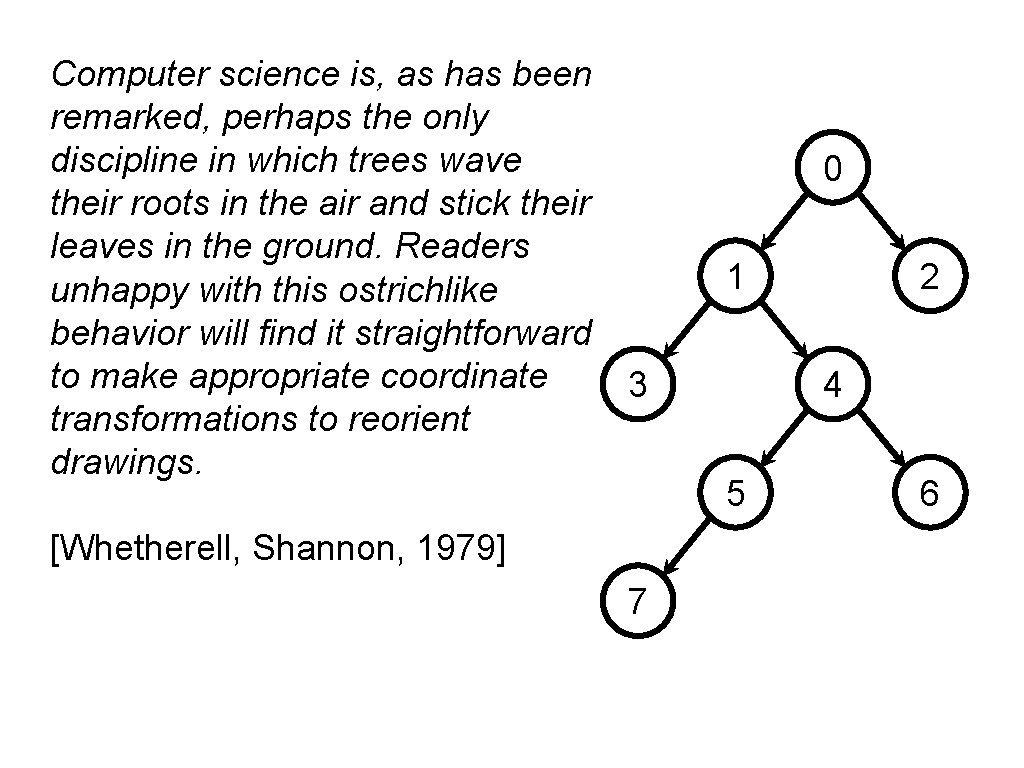
Computer science is, as has been remarked, perhaps the only discipline in which trees wave their roots in the air and stick their leaves in the ground. Readers unhappy with this ostrichlike behavior will find it straightforward to make appropriate coordinate transformations to reorient drawings. 0 1 3 4 5 [Whetherell, Shannon, 1979] 7 2 6

Arthur Cayley [Digitized by Google] [Wikipedia, Public Domain] British Mathematician 1821 – 1895 On theory of the analytical forms called trees, Philosophical Magazine, 4 th series, 13 : 172– 176, 1857. 4

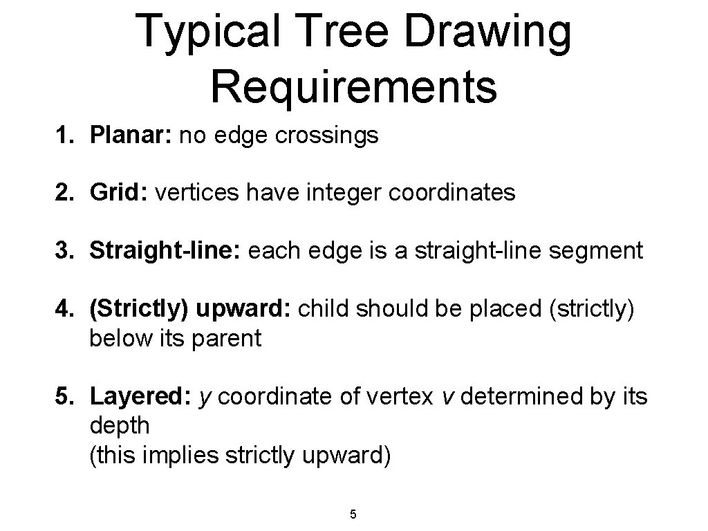
Typical Tree Drawing Requirements 1. Planar: no edge crossings 2. Grid: vertices have integer coordinates 3. Straight-line: each edge is a straight-line segment 4. (Strictly) upward: child should be placed (strictly) below its parent 5. Layered: y coordinate of vertex v determined by its depth (this implies strictly upward) 5

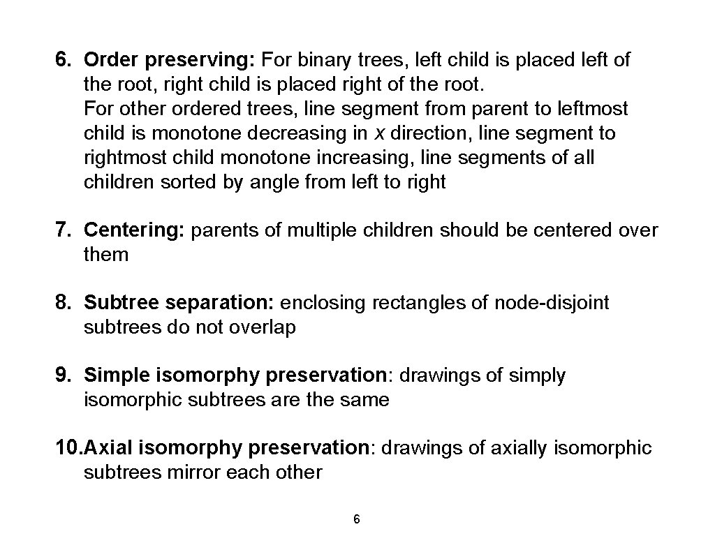
6. Order preserving: For binary trees, left child is placed left of the root, right child is placed right of the root. For other ordered trees, line segment from parent to leftmost child is monotone decreasing in x direction, line segment to rightmost child monotone increasing, line segments of all children sorted by angle from left to right 7. Centering: parents of multiple children should be centered over them 8. Subtree separation: enclosing rectangles of node-disjoint subtrees do not overlap 9. Simple isomorphy preservation: drawings of simply isomorphic subtrees are the same 10. Axial isomorphy preservation: drawings of axially isomorphic subtrees mirror each other 6

Tree Drawing Algorithm Classes 1. Layered Drawing 2. Radial Drawing 3. HV-Drawing 4. Recursive Winding 7

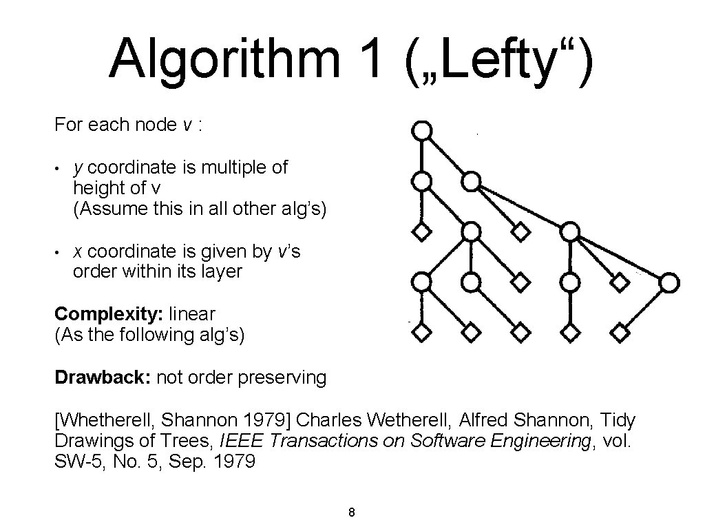
Algorithm 1 („Lefty“) For each node v : • y coordinate is multiple of height of v (Assume this in all other alg’s) • x coordinate is given by v’s order within its layer Complexity: linear (As the following alg’s) Drawback: not order preserving [Whetherell, Shannon 1979] Charles Wetherell, Alfred Shannon, Tidy Drawings of Trees, IEEE Transactions on Software Engineering, vol. SW-5, No. 5, Sep. 1979 8

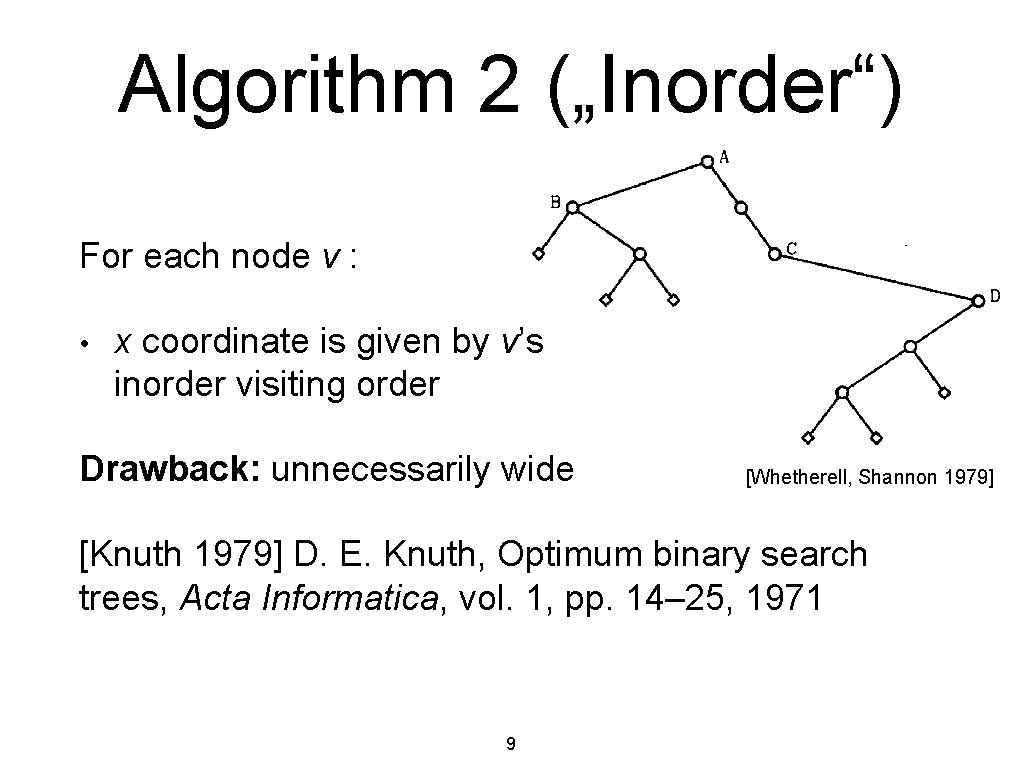
Algorithm 2 („Inorder“) For each node v : • x coordinate is given by v’s inorder visiting order Drawback: unnecessarily wide [Whetherell, Shannon 1979] [Knuth 1979] D. E. Knuth, Optimum binary search trees, Acta Informatica, vol. 1, pp. 14– 25, 1971 9

Algorithm 2 („In-Order“) [Whetherell, Shannon 1979] Best drawing In-order drawing 10

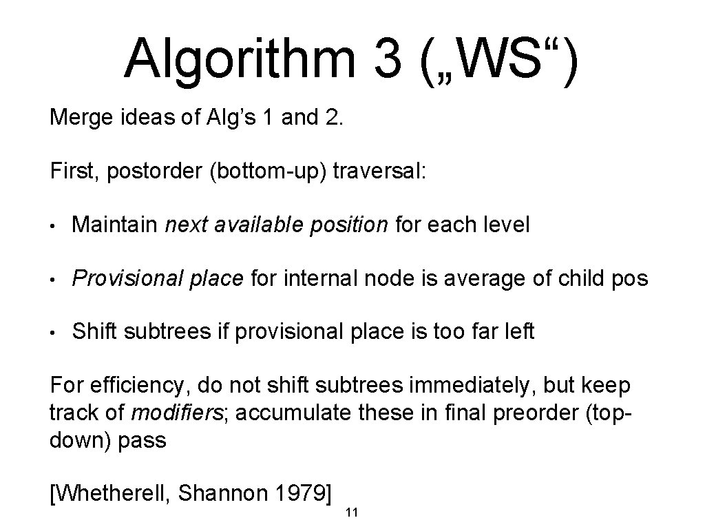
Algorithm 3 („WS“) Merge ideas of Alg’s 1 and 2. First, postorder (bottom-up) traversal: • Maintain next available position for each level • Provisional place for internal node is average of child pos • Shift subtrees if provisional place is too far left For efficiency, do not shift subtrees immediately, but keep track of modifiers; accumulate these in final preorder (topdown) pass [Whetherell, Shannon 1979] 11

Algorithm 3 („WS“) < x, modifier > [Whetherell, Shannon 1979]

Algorithm 3 („WS“) Drawback: unnecessarily wide [Reingold, Tilford 1981] 13

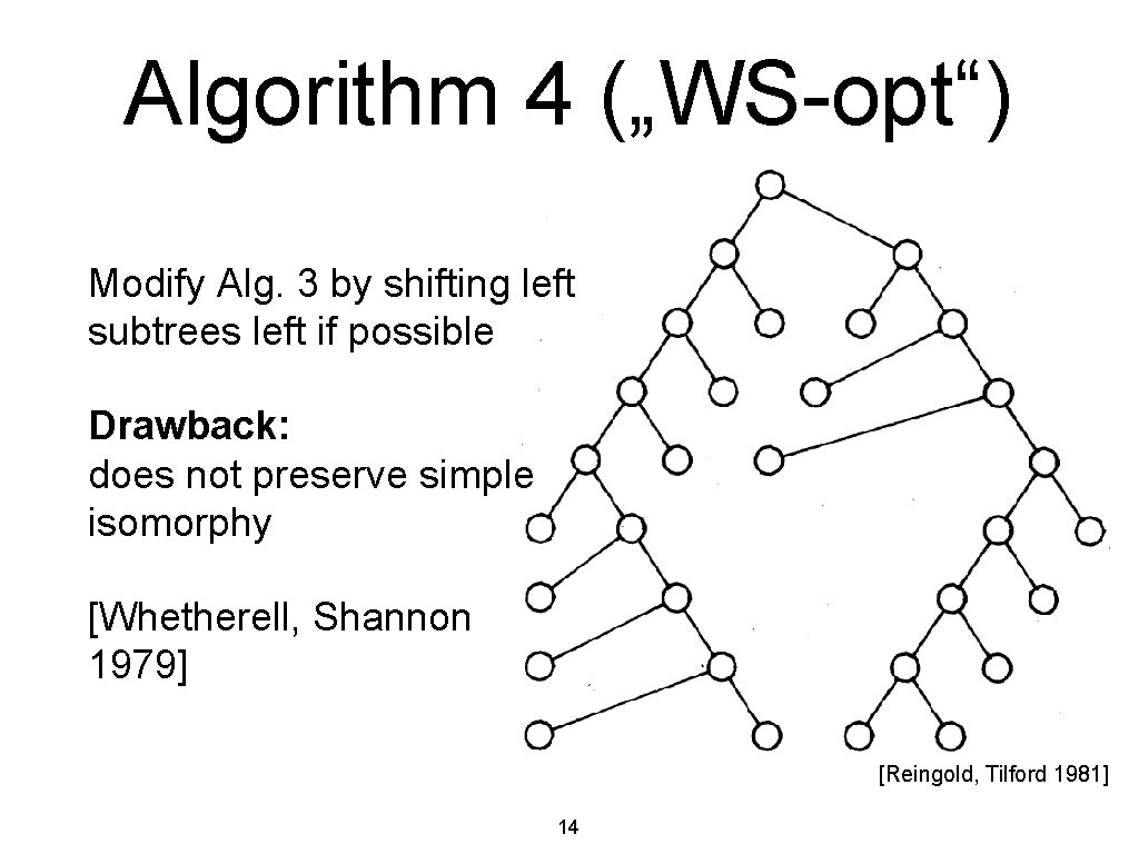
Algorithm 4 („WS-opt“) Modify Alg. 3 by shifting left subtrees left if possible Drawback: does not preserve simple isomorphy [Whetherell, Shannon 1979] [Reingold, Tilford 1981] 14

Algorithm 3 („WS“) Drawback: does not preserve axial isomorphy [Reingold, Tilford 1981] 15

Isomorphy Preservation vs. Minimum Width [Reingold, Tilford 1981] 16

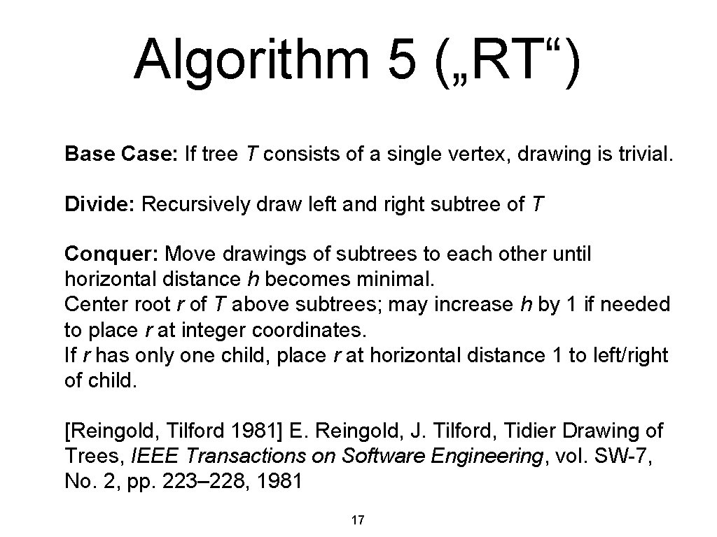
Algorithm 5 („RT“) Base Case: If tree T consists of a single vertex, drawing is trivial. Divide: Recursively draw left and right subtree of T Conquer: Move drawings of subtrees to each other until horizontal distance h becomes minimal. Center root r of T above subtrees; may increase h by 1 if needed to place r at integer coordinates. If r has only one child, place r at horizontal distance 1 to left/right of child. [Reingold, Tilford 1981] E. Reingold, J. Tilford, Tidier Drawing of Trees, IEEE Transactions on Software Engineering, vol. SW-7, No. 2, pp. 223– 228, 1981 17

18 [Reingold, Tilford 1981]

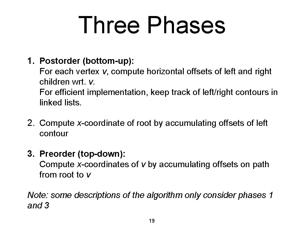
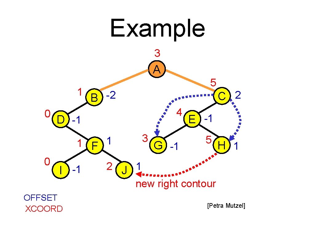
Three Phases 1. Postorder (bottom-up): For each vertex v, compute horizontal offsets of left and right children wrt. v. For efficient implementation, keep track of left/right contours in linked lists. 2. Compute x-coordinate of root by accumulating offsets of left contour 3. Preorder (top-down): Compute x-coordinates of v by accumulating offsets on path from root to v Note: some descriptions of the algorithm only consider phases 1 and 3 19

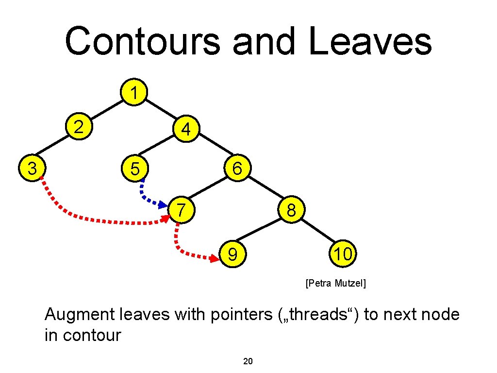
Contours and Leaves 1 2 3 4 6 5 8 7 10 9 [Petra Mutzel] Augment leaves with pointers („threads“) to next node in contour 20

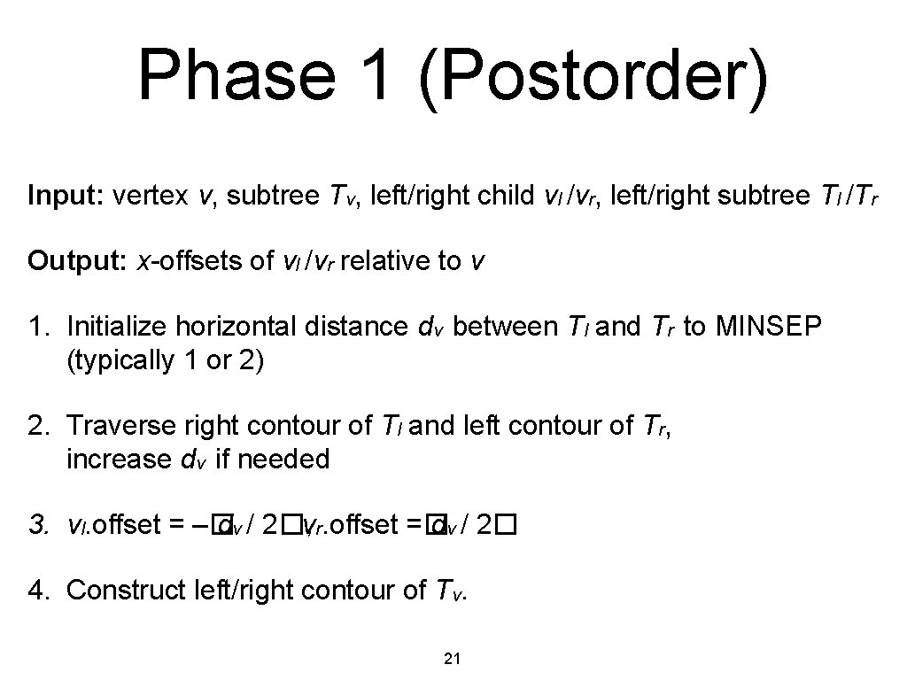
Phase 1 (Postorder) Input: vertex v, subtree Tv, left/right child vl /vr, left/right subtree Tl /Tr Output: x-offsets of vl /vr relative to v 1. Initialize horizontal distance dv between Tl and Tr to MINSEP (typically 1 or 2) 2. Traverse right contour of Tl and left contour of Tr, increase dv if needed 3. vl. offset = –� dv / 2�, vr. offset =� dv / 2� 4. Construct left/right contour of Tv. 21

Example 3 A 1 0 5 B -2 4 D -1 1 F 0 C 2 I -1 OFFSET XCOORD 1 3 G -1 E -1 5 H 1 2 J 1 new right contour [Petra Mutzel]

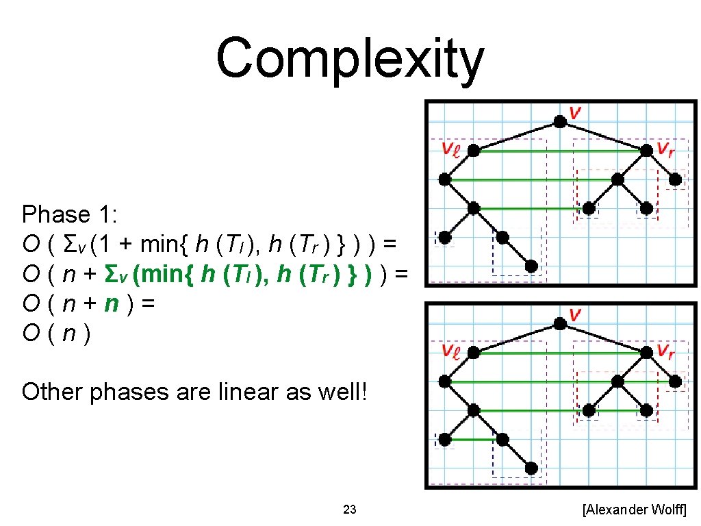
Complexity Phase 1: O ( Σv (1 + min{ h (Tl ), h (Tr ) } ) ) = O ( n + Σv (min{ h (Tl ), h (Tr ) } ) ) = O(n+n)= O(n) Other phases are linear as well! 23 [Alexander Wolff]

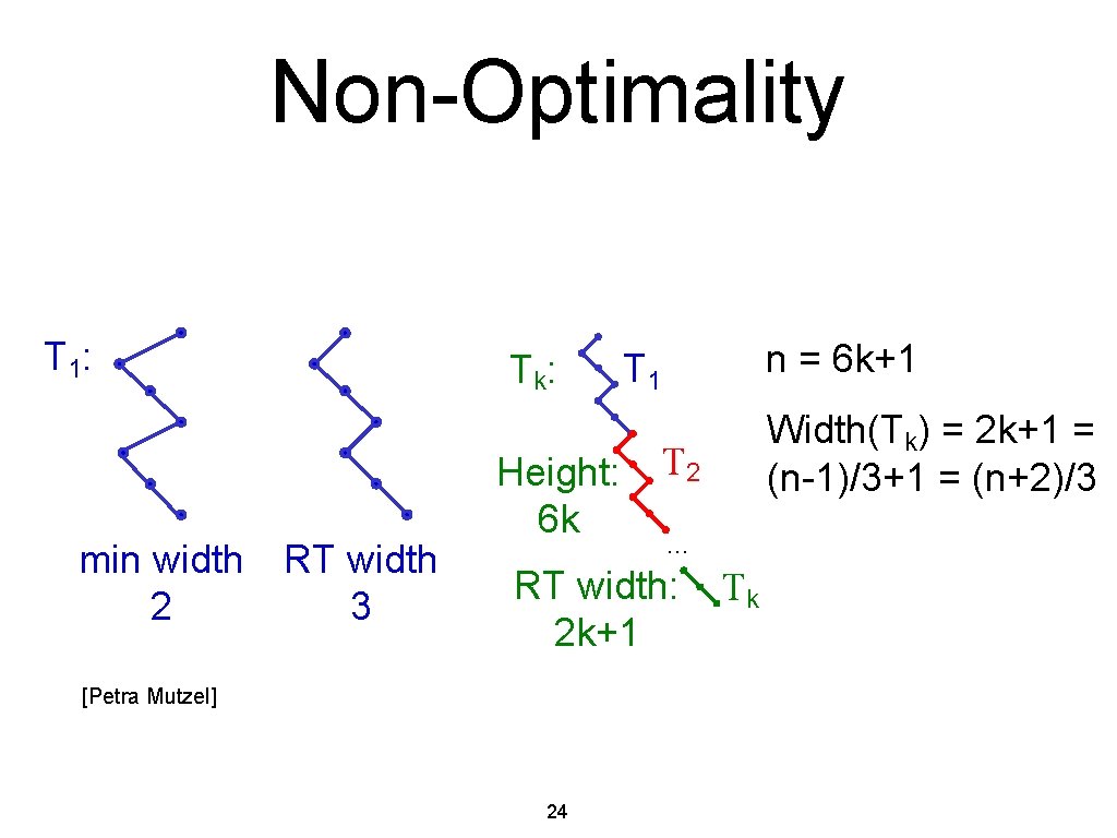
Non-Optimality T 1: min width RT width 2 3 Tk: Height: 6 k n = 6 k+1 T 2 … RT width: 2 k+1 [Petra Mutzel] 24 Width(Tk) = 2 k+1 = (n-1)/3+1 = (n+2)/3 Tk

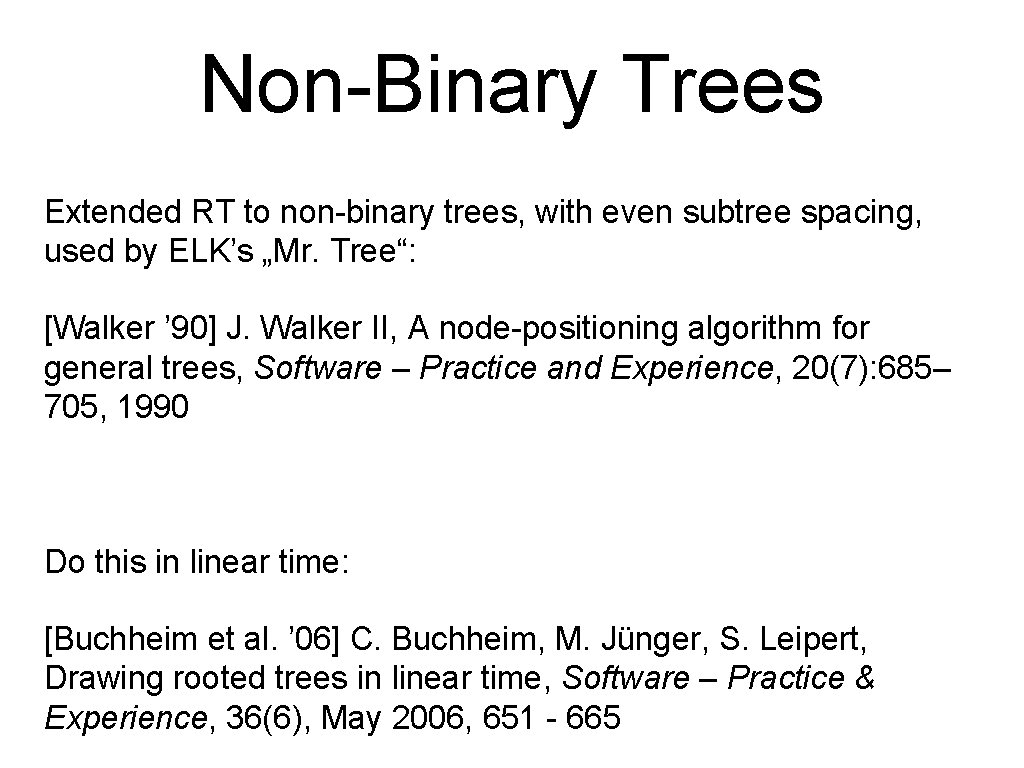
Non-Binary Trees Extended RT to non-binary trees, with even subtree spacing, used by ELK’s „Mr. Tree“: [Walker ’ 90] J. Walker II, A node-positioning algorithm for general trees, Software – Practice and Experience, 20(7): 685– 705, 1990 Do this in linear time: [Buchheim et al. ’ 06] C. Buchheim, M. Jünger, S. Leipert, Drawing rooted trees in linear time, Software – Practice & Experience, 36(6), May 2006, 651 - 665

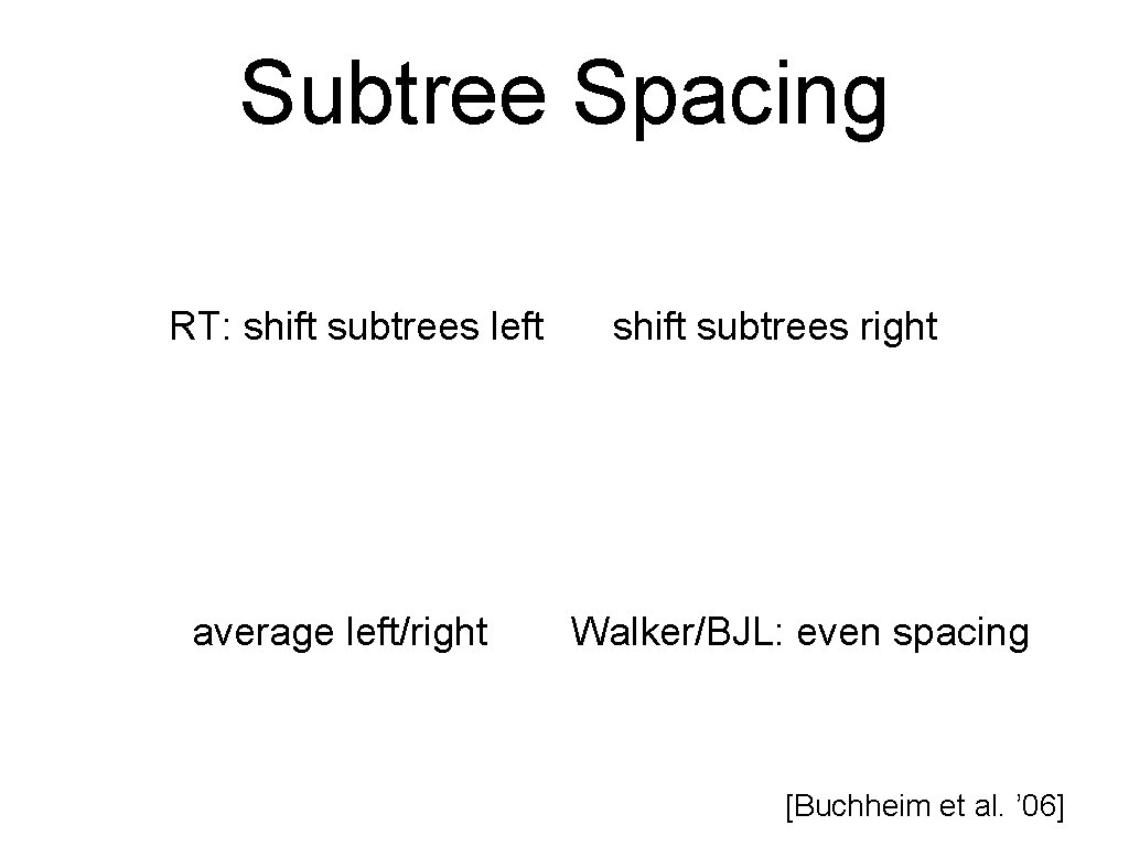
Subtree Spacing RT: shift subtrees left average left/right shift subtrees right Walker/BJL: even spacing [Buchheim et al. ’ 06]

Spacing Smaller Subtrees [Buchheim et al. ’ 06]

shift change Computing Shifts shift change [Buchheim et al. ’ 06]

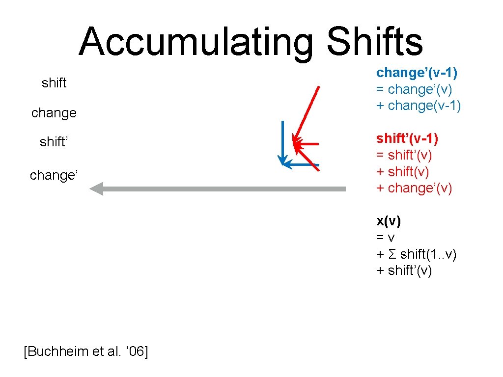
Accumulating Shifts shift change shift’ change’(v-1) = change’(v) + change(v-1) shift’(v-1) = shift’(v) + shift(v) + change’(v) x(v) =v + Σ shift(1. . v) + shift’(v) [Buchheim et al. ’ 06]

Tree Drawing Algorithm Classes 1. Layered Drawing 2. Radial Drawing 3. HV-Drawing 4. Recursive Winding [Eades ’ 92] Peter Eades, Drawing Free Trees, Bulletin of the ICA, vol. 5, 1992, pp. 10– 36 30

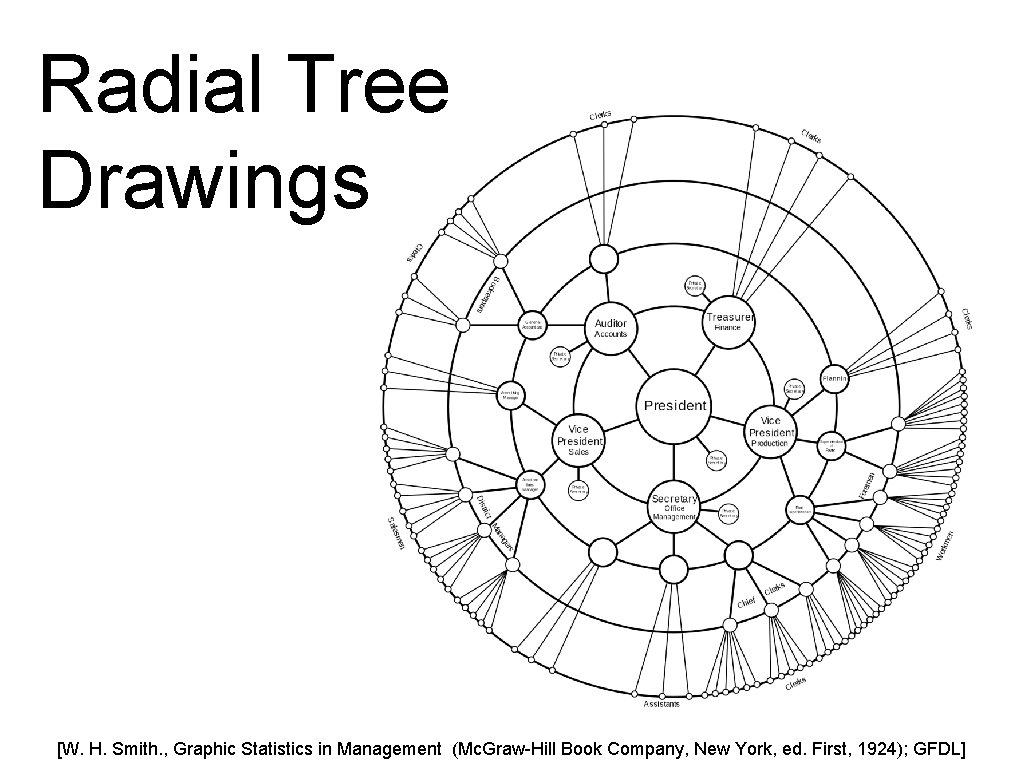
Radial Tree Drawings [W. H. Smith. , Graphic Statistics in Management (Mc. Graw-Hill Book Company, New York, ed. First, 1924); GFDL]

A Simple Algorithm [Alexander Wolff]

Limit Sectors Annulus wedge [Alexander Wolff]

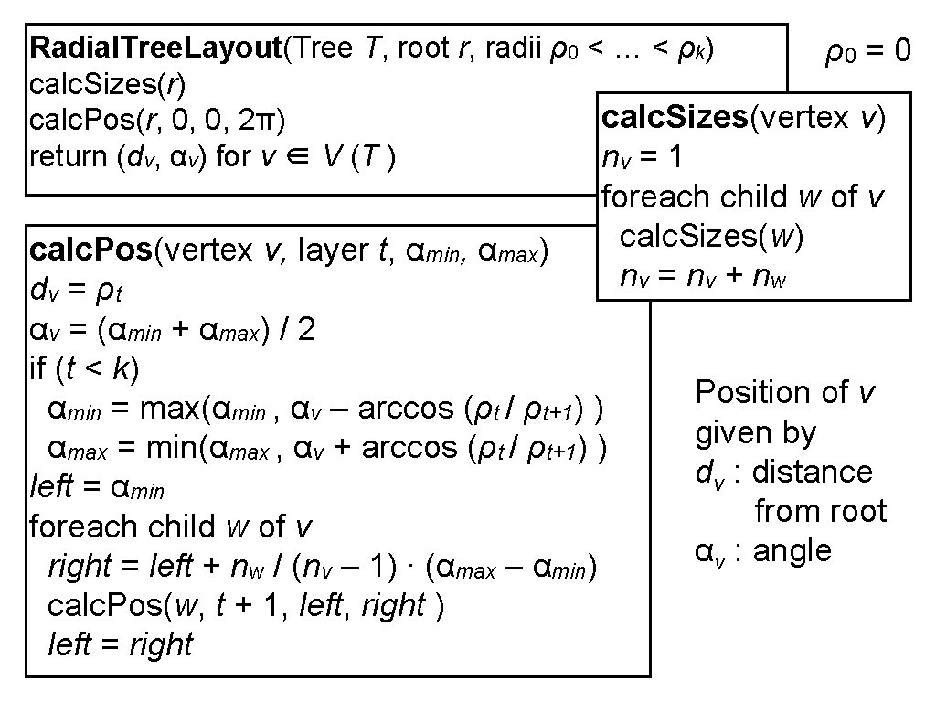
Radial. Tree. Layout(Tree T, root r, radii ρ0 < … < ρk) ρ0 = 0 calc. Sizes(r) calc. Sizes(vertex v) calc. Pos(r, 0, 0, 2π) return (dv, αv) for v ∈ V (T ) nv = 1 foreach child w of v calc. Sizes(w) nv = nv + n w calc. Pos(vertex v, layer t, αmin, αmax) dv = ρ t αv = (αmin + αmax) / 2 if (t < k) αmin = max(αmin , αv – arccos (ρt / ρt+1) ) αmax = min(αmax , αv + arccos (ρt / ρt+1) ) left = αmin foreach child w of v right = left + nw / (nv – 1) ∙ (αmax – αmin) calc. Pos(w, t + 1, left, right ) left = right Position of v given by dv : distance from root αv : angle

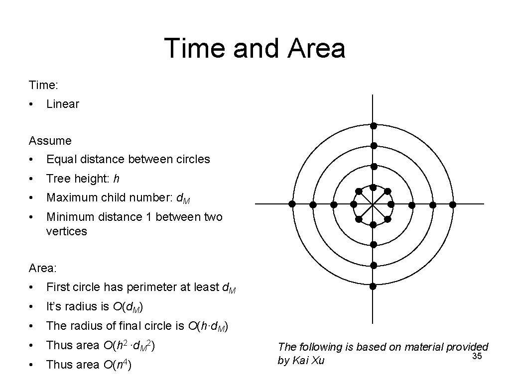
Time and Area Time: • Linear Assume • Equal distance between circles • Tree height: h • Maximum child number: d. M • Minimum distance 1 between two vertices Area: • First circle has perimeter at least d. M • It’s radius is O(d. M) • The radius of final circle is O(h∙d. M) • Thus area O(h 2 ∙d. M 2) • Thus area O(n 4) The following is based on material provided 35 by Kai Xu

Radial Drawing Used for free trees (tree without a root) • Select a root that minimizes tree height • Can be found in linear time using simple recursive leaf pruning algorithm • Results in one or two centers Variations: • Choice of root • Radii of the circles • How to determine the wedge angle 36

Tree Drawing Algorithm Classes 1. Layered Drawing 2. Radial Drawing 3. HV-Drawing 4. Recursive Winding [Crescenzi et al. '92] P. Crescenzi, G. Di Battista, A. Piperno, A note on optimal area algorithms for upward drawings of binary trees, Computational Geometry, 2 (4), Dec. 1992, 187– 200 37

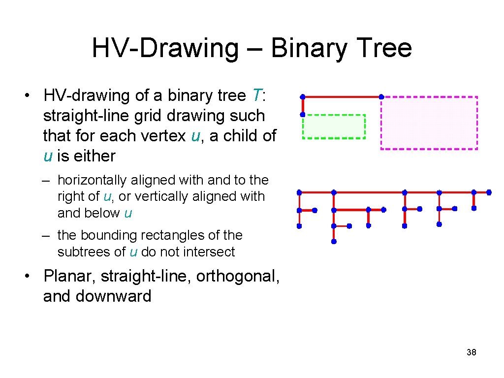
HV-Drawing – Binary Tree • HV-drawing of a binary tree T: straight-line grid drawing such that for each vertex u, a child of u is either – horizontally aligned with and to the right of u, or vertically aligned with and below u – the bounding rectangles of the subtrees of u do not intersect • Planar, straight-line, orthogonal, and downward 38

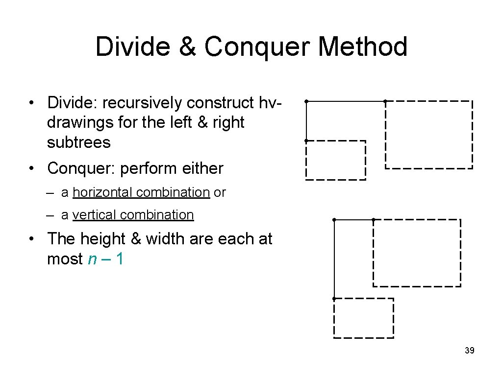
Divide & Conquer Method • Divide: recursively construct hvdrawings for the left & right subtrees • Conquer: perform either – a horizontal combination or – a vertical combination • The height & width are each at most n – 1 39

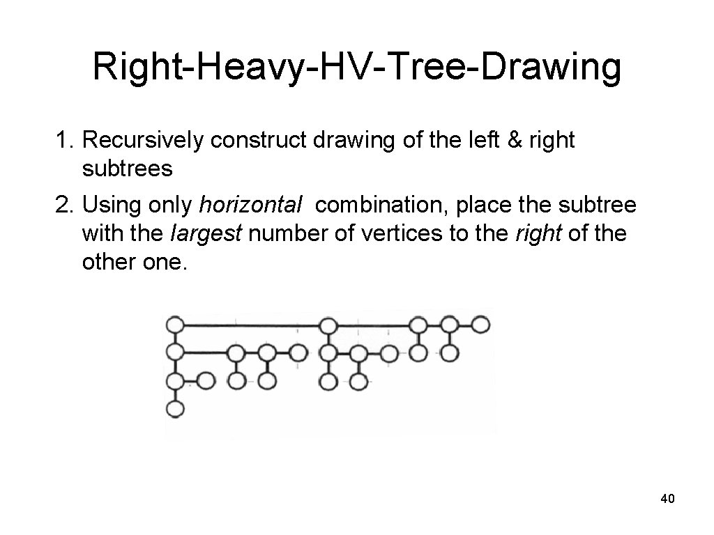
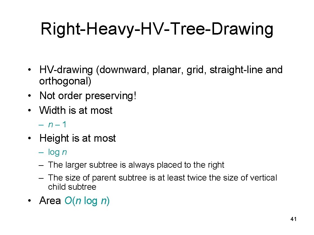
Right-Heavy-HV-Tree-Drawing 1. Recursively construct drawing of the left & right subtrees 2. Using only horizontal combination, place the subtree with the largest number of vertices to the right of the other one. height of the drawing is at most logn 40

Right-Heavy-HV-Tree-Drawing • HV-drawing (downward, planar, grid, straight-line and orthogonal) • Not order preserving! • Width is at most – n– 1 • Height is at most – log n – The larger subtree is always placed to the right – The size of parent subtree is at least twice the size of vertical child subtree • Area O(n log n) 41

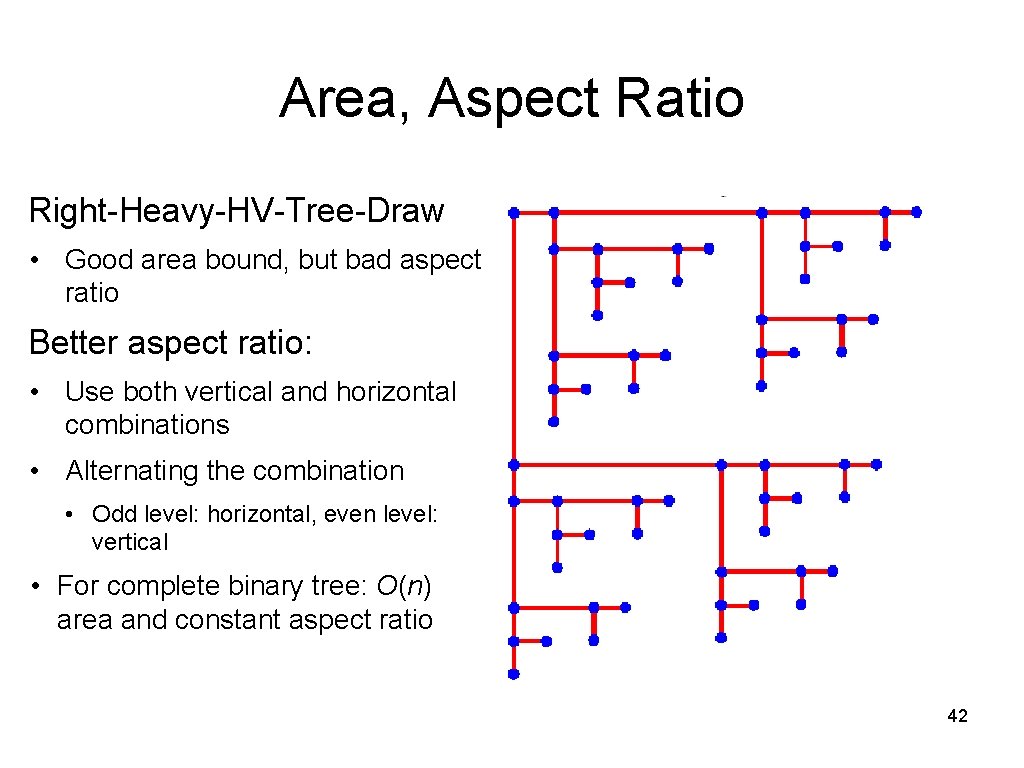
Area, Aspect Ratio Right-Heavy-HV-Tree-Draw • Good area bound, but bad aspect ratio Better aspect ratio: • Use both vertical and horizontal combinations • Alternating the combination • Odd level: horizontal, even level: vertical • For complete binary tree: O(n) area and constant aspect ratio 42

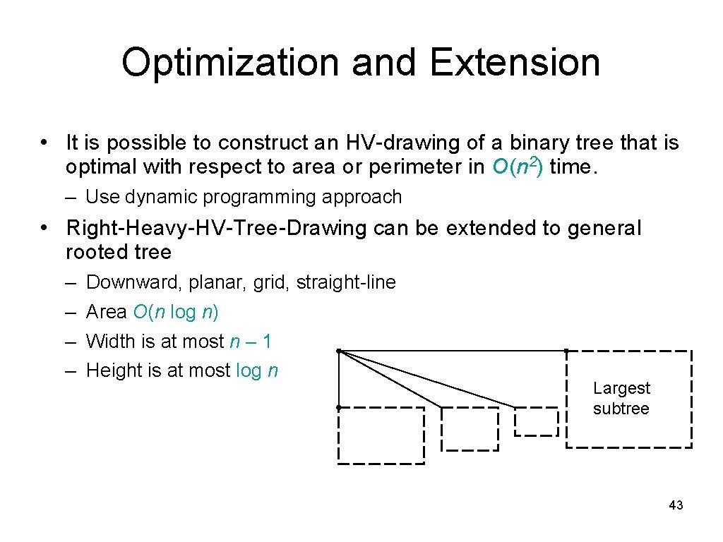
Optimization and Extension • It is possible to construct an HV-drawing of a binary tree that is optimal with respect to area or perimeter in O(n 2) time. – Use dynamic programming approach • Right-Heavy-HV-Tree-Drawing can be extended to general rooted tree – – Downward, planar, grid, straight-line Area O(n log n) Width is at most n – 1 Height is at most log n Largest subtree 43

Tree Visualization • While tree drawing algorithm is more theoretical, tree visualization is more applied. • We will see examples of different tree visualization methods. 52

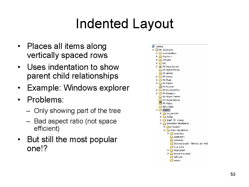
Indented Layout • Places all items along vertically spaced rows • Uses indentation to show parent child relationships • Example: Windows explorer • Problems: – Only showing part of the tree – Bad aspect ratio (not space efficient) • But still the most popular one!? 53

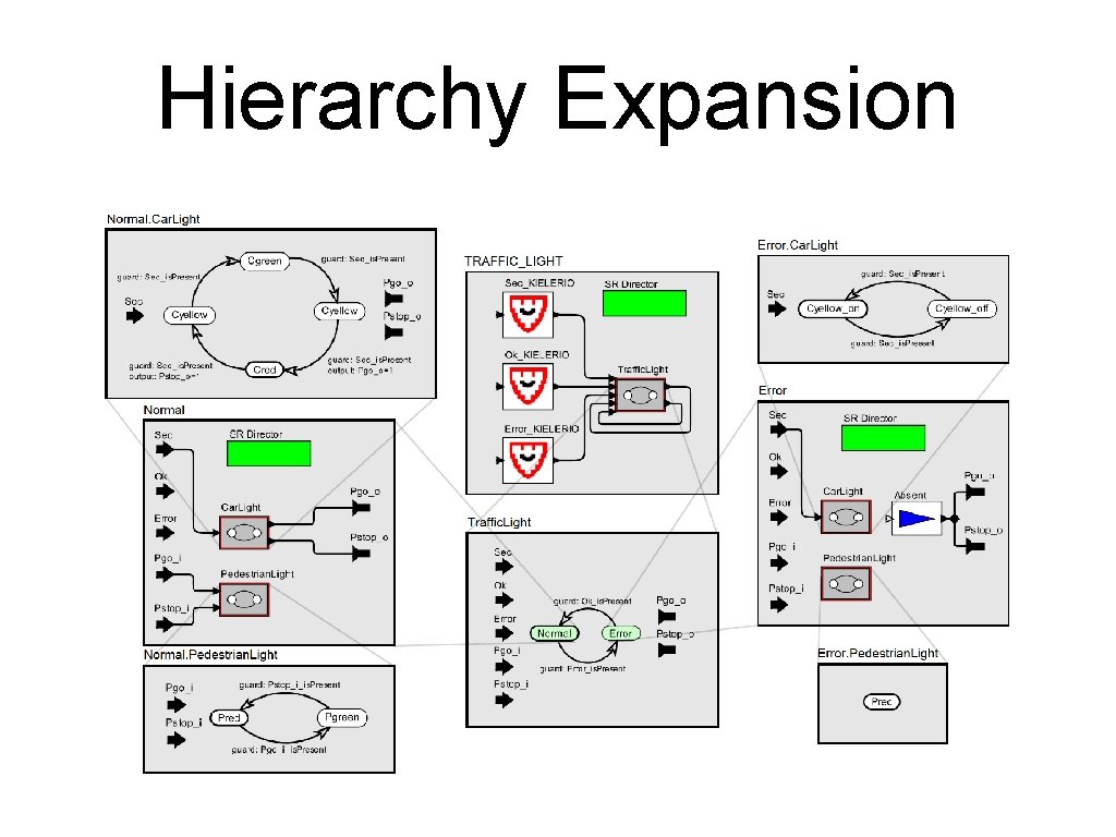
Hierarchy Expansion

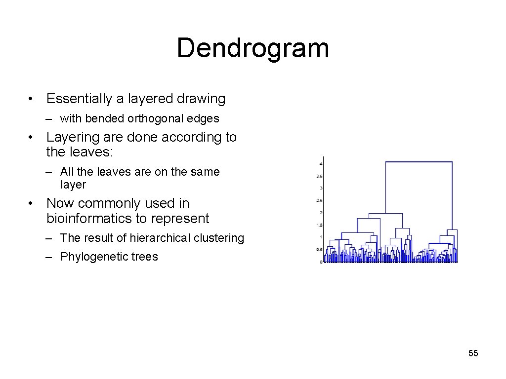
Dendrogram • Essentially a layered drawing – with bended orthogonal edges • Layering are done according to the leaves: – All the leaves are on the same layer • Now commonly used in bioinformatics to represent – The result of hierarchical clustering – Phylogenetic trees 55

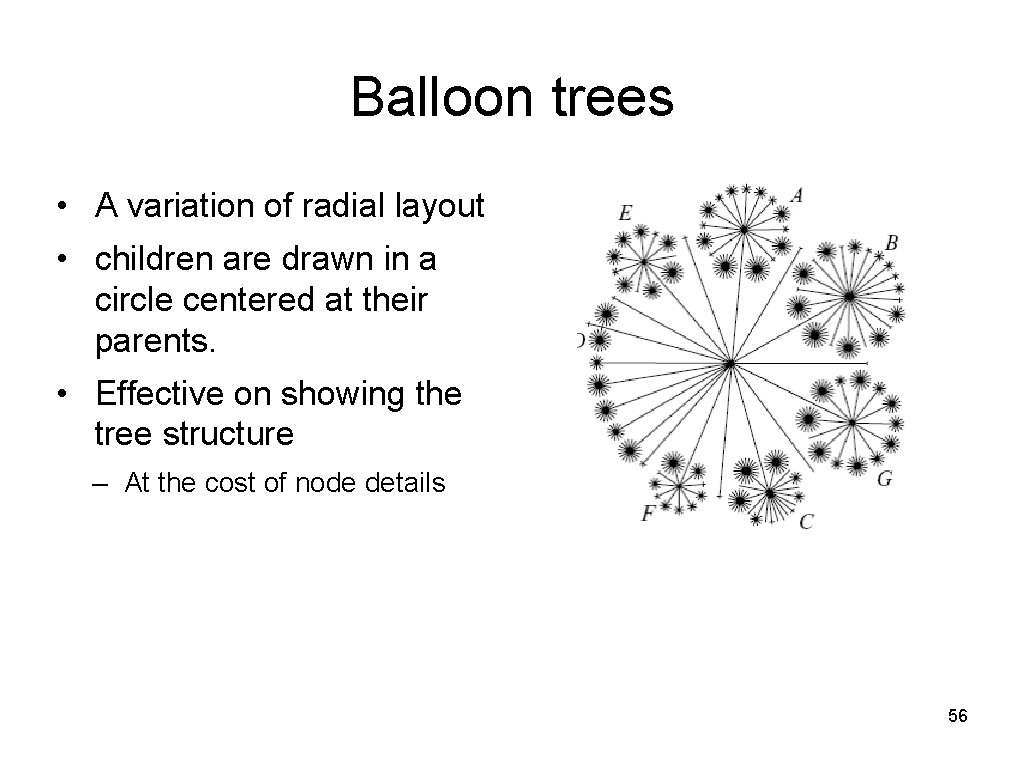
Balloon trees • A variation of radial layout • children are drawn in a circle centered at their parents. • Effective on showing the tree structure – At the cost of node details 56

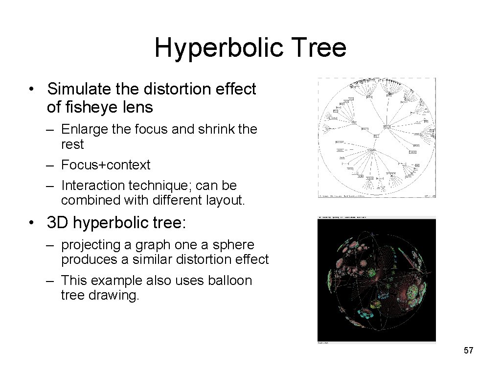
Hyperbolic Tree • Simulate the distortion effect of fisheye lens – Enlarge the focus and shrink the rest – Focus+context – Interaction technique; can be combined with different layout. • 3 D hyperbolic tree: – projecting a graph one a sphere produces a similar distortion effect – This example also uses balloon tree drawing. 57

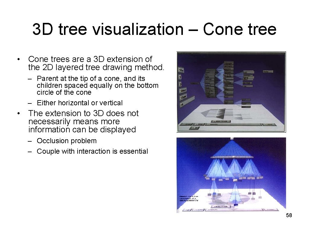
3 D tree visualization – Cone tree • Cone trees are a 3 D extension of the 2 D layered tree drawing method. – Parent at the tip of a cone, and its children spaced equally on the bottom circle of the cone – Either horizontal or vertical • The extension to 3 D does not necessarily means more information can be displayed – Occlusion problem – Couple with interaction is essential 58

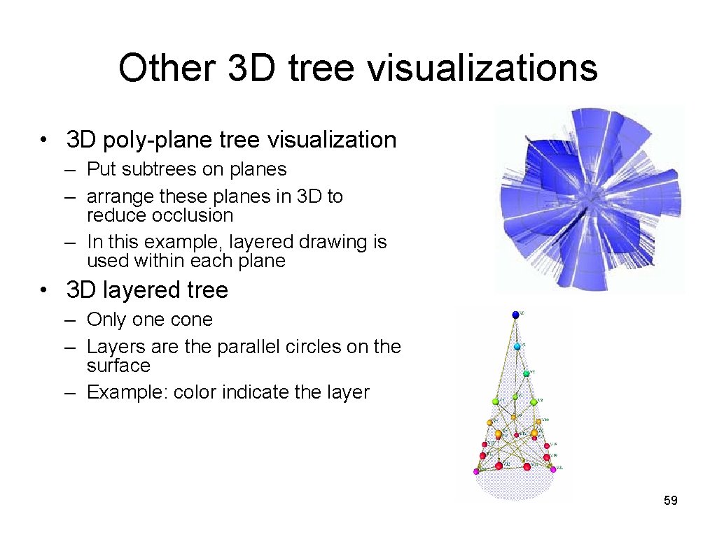
Other 3 D tree visualizations • 3 D poly-plane tree visualization – Put subtrees on planes – arrange these planes in 3 D to reduce occlusion – In this example, layered drawing is used within each plane • 3 D layered tree – Only one cone – Layers are the parallel circles on the surface – Example: color indicate the layer 59

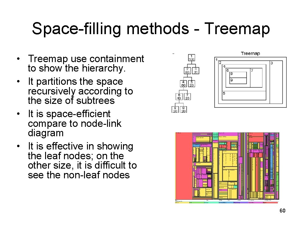
Space-filling methods - Treemap • Treemap use containment to show the hierarchy. • It partitions the space recursively according to the size of subtrees • It is space-efficient compare to node-link diagram • It is effective in showing the leaf nodes; on the other size, it is difficult to see the non-leaf nodes 60

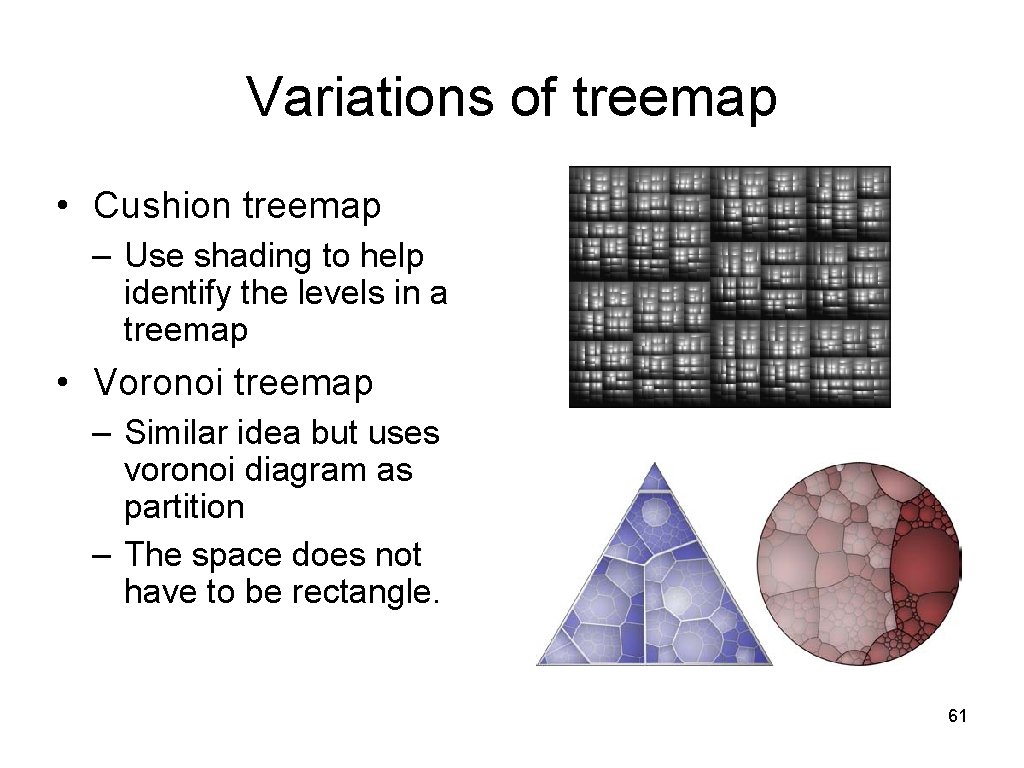
Variations of treemap • Cushion treemap – Use shading to help identify the levels in a treemap • Voronoi treemap – Similar idea but uses voronoi diagram as partition – The space does not have to be rectangle. 61

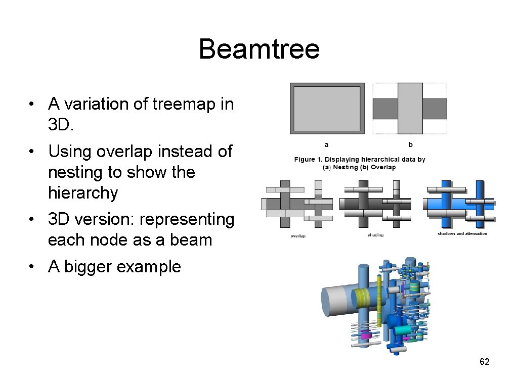
Beamtree • A variation of treemap in 3 D. • Using overlap instead of nesting to show the hierarchy • 3 D version: representing each node as a beam • A bigger example 62

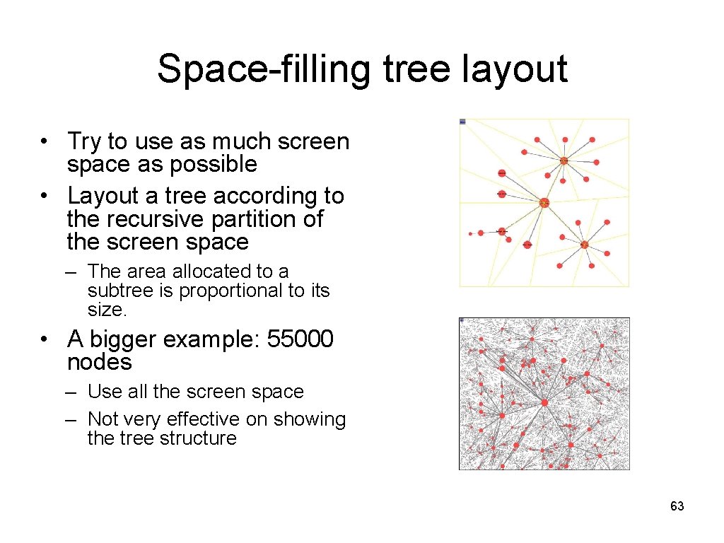
Space-filling tree layout • Try to use as much screen space as possible • Layout a tree according to the recursive partition of the screen space – The area allocated to a subtree is proportional to its size. • A bigger example: 55000 nodes – Use all the screen space – Not very effective on showing the tree structure 63

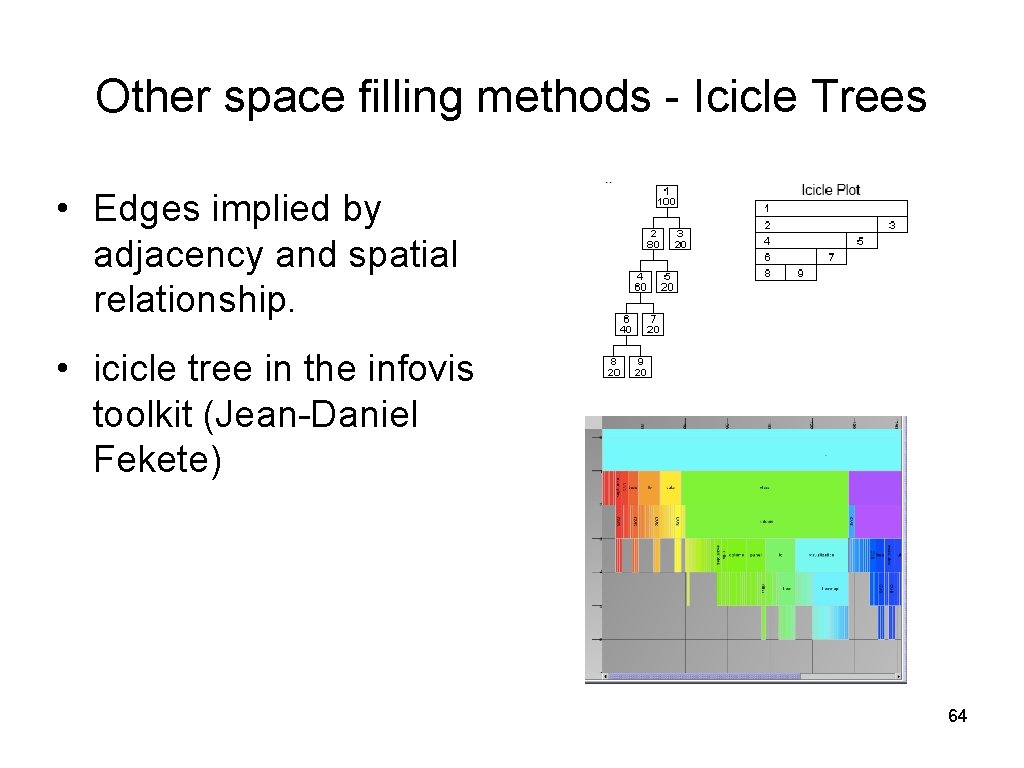
Other space filling methods - Icicle Trees • Edges implied by adjacency and spatial relationship. • icicle tree in the infovis toolkit (Jean-Daniel Fekete) 64

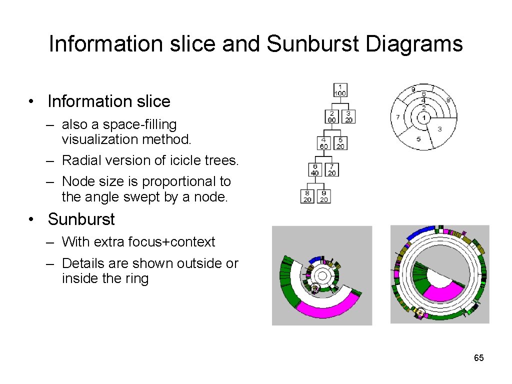
Information slice and Sunburst Diagrams • Information slice – also a space-filling visualization method. – Radial version of icicle trees. – Node size is proportional to the angle swept by a node. • Sunburst – With extra focus+context – Details are shown outside or inside the ring 65

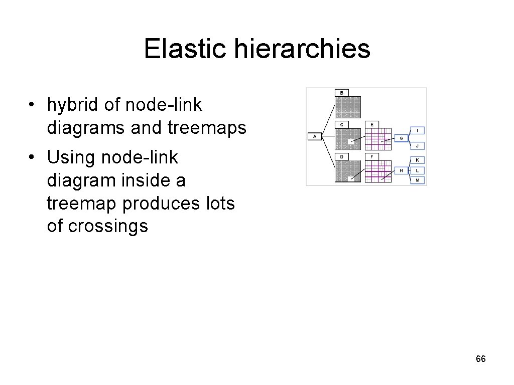
Elastic hierarchies • hybrid of node-link diagrams and treemaps • Using node-link diagram inside a treemap produces lots of crossings 66

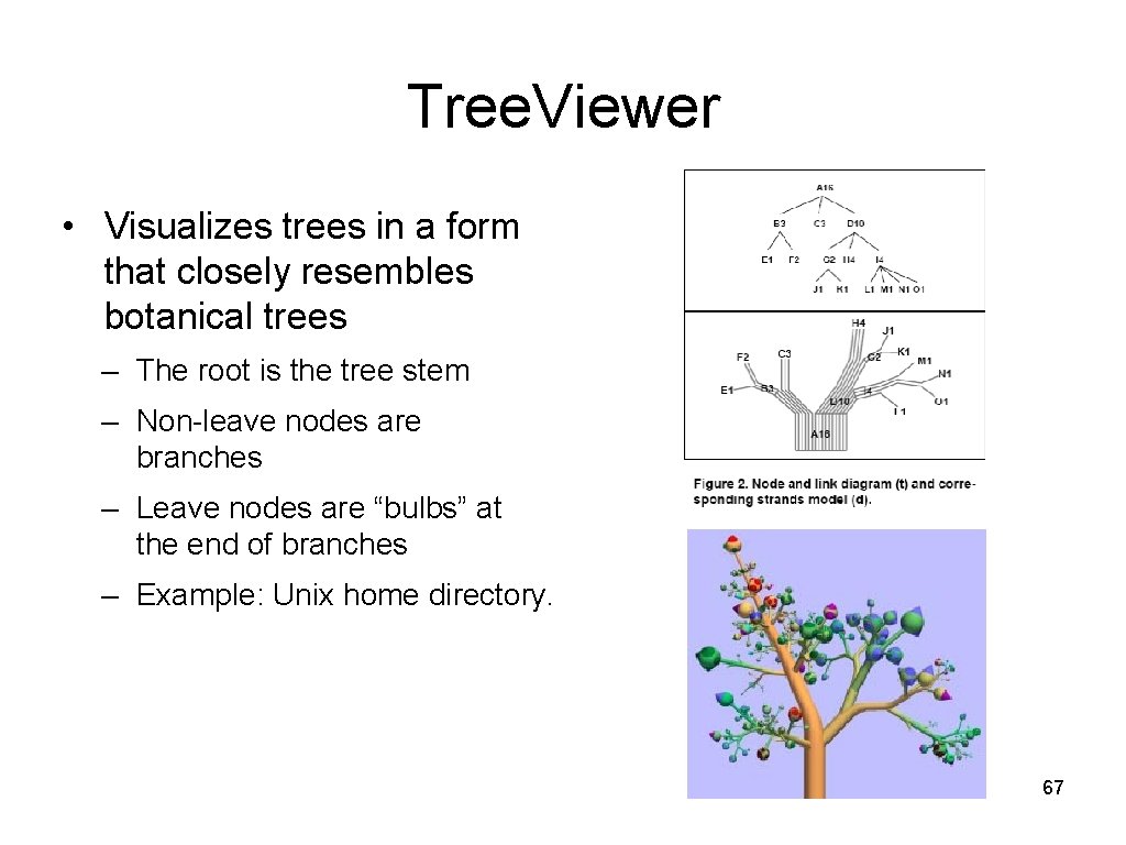
Tree. Viewer • Visualizes trees in a form that closely resembles botanical trees – The root is the tree stem – Non-leave nodes are branches – Leave nodes are “bulbs” at the end of branches – Example: Unix home directory. 67

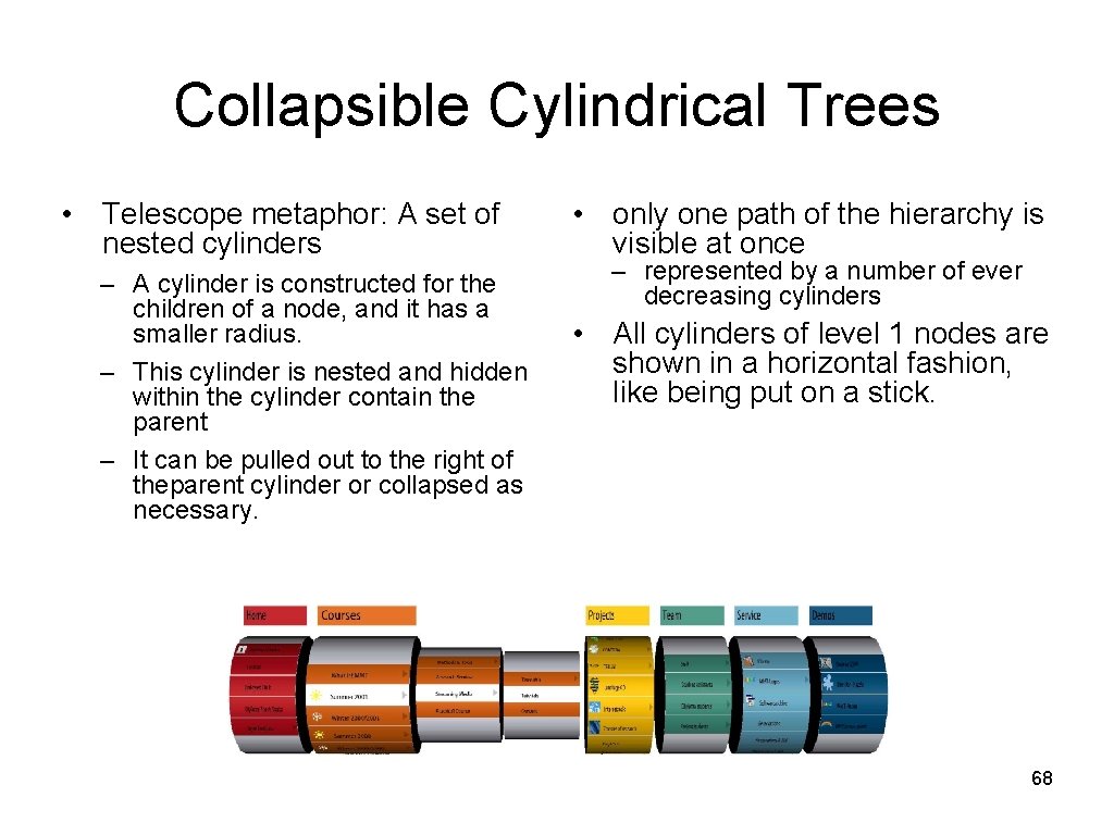
Collapsible Cylindrical Trees • Telescope metaphor: A set of nested cylinders – A cylinder is constructed for the children of a node, and it has a smaller radius. – This cylinder is nested and hidden within the cylinder contain the parent – It can be pulled out to the right of theparent cylinder or collapsed as necessary. • only one path of the hierarchy is visible at once – represented by a number of ever decreasing cylinders • All cylinders of level 1 nodes are shown in a horizontal fashion, like being put on a stick. 68

Summary • Typical tree drawing requirements: planar, on a grid, straight-line, upward/layered, order preserving, … • There exist a variety of layered drawings, most of them efficient (linear complexity); it’s non-trivial to preserve isomorphy • Radial drawings may suffer from non-planarity • Horizontal-vertical drawings may produce compact drawings, at the cost of order preservation • There are numerous additional ways to visualize trees 69