Inferential Statistics Dr Mohammed Alahmed Ph D in

Inferential Statistics Dr. Mohammed Alahmed Ph. D. in Bio. Statistics alahmed@ksu. edu. sa (011) 4674108

Descriptive statistics Estimation Statistics Inferential statistics Hypothesis Testing Modeling, Predicting 2

3

Inferential Statistics Statistical inference is the act of generalizing from a sample to a population with calculated degree of certainty. We want to learn about population parameters… but we can only calculate sample statistics Methods for drawing conclusions about a population from sample data are called 4

Parameters and Statistics It is essential that we draw distinctions between parameters and statistics 5

Population (parameters, e. g. , and ) Sample collect data from individuals in sample Data Analyse data (e. g. estimate ) to make inferences 6

Estimation That act of guessing the value of a population parameter Point Estimation Estimating a specific value Interval Estimation determining the range or interval in which the value of the parameter is thought to be 7

Introduction • The objective of estimation is to determine the approximate value of a population parameter on the basis of a sample statistic. • One of our fundamental questions is: “How well does our sample statistic estimate the value of the population parameter? ” • In other word: How close is Sample Statistic to Population Parameter ? 8

• A point estimate draws inferences about a population by estimating the value of an unknown parameter using a single value or point. – How much uncertainty is associated with a point estimate of a population parameter? • An interval estimate provides more information about a population characteristic than does a point estimate. It provides a confidence level for the estimate. Such interval estimates are called confidence intervals. Lower Confidence Limit Upper Point Estimate Confidence Limit Width of confidence interval 9

• A confidence interval for a population characteristic is an interval of plausible values for the characteristic. It is constructed so that, with a chosen degree of confidence (the confidence level), the value of the characteristic will be captured inside the interval • Confidence in statistics is a measure of our guaranty that a key value falls within a specified interval. • A Confidence Interval is always accompanied by a probability that defines the risk of being wrong. • This probability of error is usually called α (alpha). 10

• How confident do we want to be that the interval estimate contains the population parameter? • The level of confidence (1 - α ) is the probability that the interval estimate contains the population parameter. • The most common choices of level of confidence are 0. 95, 0. 99, and 0. 90. • For example: If the level of confidence is 90%, this means that we are 90% confident that the interval contains the population parameter. • The general formula for all confidence intervals is equal to: Point Estimate ± Margin of Error 11

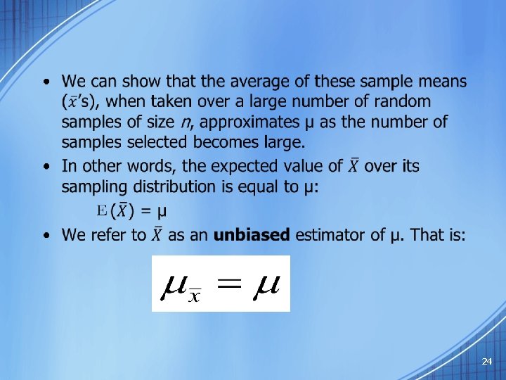
Choosing a good estimator Good estimators have certain desirable properties: • Unbiasedness: The sampling distribution for the estimator ‘centers’ around the parameter. (On average, the estimator gives the correct value for the parameter. ) • Efficiency: If at the sample size one unbiased estimator has a smaller sampling error than another unbiased estimator, the first one is more efficient. • Consistency: The value of the estimator gets closer to the parameter as sample size increases. Consistent estimators may be biased, but the bias must become smaller as the sample size increases if the consistency property holds true. 12

Sampling Distribution • 13

Central Limit Theorem For any population with mean and standard deviation , the distribution of sample means for sample size n … 1. will have a mean of 2. will have a standard deviation(standard error) of 3. will approach a normal distribution as n gets large ( n ≥ 30 ). 14

Example Given the population of women has normally distributed weights with a mean of 143 lbs and a standard deviation of 29 lbs, 1. if one woman is randomly selected, find the probability that her weight is greater than 150 lbs. 2. if 36 different women are randomly selected, find the probability that their average weight is greater than 150 lbs. 15

1. The probability that her weight is greater than 150 lbs. z = 150 -143 = 0. 24 29 Population distribution 0. 4052 = 143 150 = 29 Z 16

2. if 36 different women are randomly selected, find the probability that their mean weight is greater than 150 lbs. Sampling distribution 0. 0735 z = 150 -143 = 1. 45 4. 83 Z = 143 150 = 4. 83 17

18

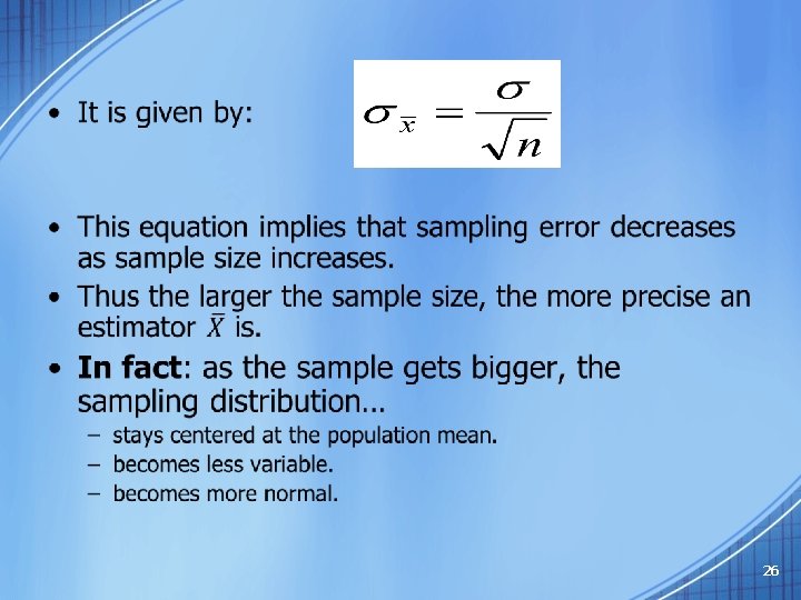
Sampling Error • Sampling error is the error caused by observing a sample instead of the whole population. • Sampling error gives us some idea of the precision of our statistical estimate. • Size of error can be measured in probability samples. • Expressed as “standard error” – of mean, proportion… • Standard error (or precision) depends upon: – size of the sample – distribution of character of interest in population 19

1. Estimating the population mean 2. Estimating the population variance σ2 3. Estimating the population proportion 20

Estimating the Population Mean • 21

The (1 - α) % confidence interval for μ is given by: • Higher confidence C implies a larger margin of error m (thus less precision in our estimates). C • A lower confidence level C produces a smaller margin of error m (thus better precision in our estimates). m −z* m z* 22

Example • 23

• Standard Error of the Mean – We can estimate how much variability there is among potential sample means by calculating the standard deviation of the mean. – Thus, it is measure of how good our point estimate is likely to be! – The standard error of the mean is the standard deviation of the sampling distribution. 25

There are 3 different cases: 1. Interval Estimation of μ when X is normally distributed. 2. Interval Estimation of μ when X is not normally distributed but the population Standard Deviation is known 3. Interval Estimation of μ when X is normally distributed and the population Standard Deviation unknown 27

Case 1: Interval Estimation of μ when X is normally distributed • This is the standard situation and you simply use this equation to estimate the population mean at the desired confidence interval: • where Z is the standard normal distribution’s critical value for a probability of α /2 in each tail. 28

Consider a 95% confidence interval: . 475 Z= -1. 96 Lower Confidence Limit μl 0 Point Estimate Z= 1. 96 Z Upper Confidence Limit μu μ 29

Case 2: Interval Estimation of μ when X is not normally distributed but σ is known • If the distribution of X is not normally distributed, then the central limit theorem can only be applied loosely and we can only say that the sampling distribution is approximately normal. • When n is greater than 30, this approximation is generally good. • Then we use the previous formula to calculate confidence interval. 30

Case 3: Interval Estimation of μ when X is normally distributed and σ is unknown • Nearly always is unknown and is estimated using sample standard deviation s. • If population standard deviation is unknown then it can be shown that sample means from samples of size n are t-distributed with n-1 degrees of freedom. • As an estimate for standard error we can use: 31

Student’s t Distribution • Closely related to the standard normal distribution Z – Symmetric and bell-shaped – Has mean = 0 but has a larger standard deviation – As n increases, the t-dist. approached the Z-dist. • Exact shape depends on a parameter called degrees of freedom (df) which is related to sample size – In this context df = n-1 32

t Table 33

• A 100% × (1 − α) CI for the mean μ of a normal distribution with unknown variance is given by: where is the critical value of the t distribution with n-1 d. f. and an area of α/2 in each tail 34

Example: Left ventricular ejection fraction (LVEF) • We have 27 patients with acute dilated cardiomyopathy. Compute a 95% CI for the true mean LVEF. 1 2 3 4 5 6 7 8 9 10 11 12 13 14 . 19. 24. 17. 40. 23. 20. 30. 19. 24. 32. 28 35

Use SPSS to do this! Analyze Descriptive Statistics Explore S = 0. 07992 36

Conclusion: We are 95% confident that the true mean of LVEF will be contained in the interval ( 0. 1925, 0. 2557) 37

Using Excel LVEF Confidence Level(95. 0%) 0. 0316 95% CI for the LVEF mean is given by: 0. 2241 ± 0. 0316 38

Estimating the population variance σ2 Point Estimation of σ2 • Let X 1, . . . , Xn be a random sample from some population with mean μ and variance σ2. • The sample variance S 2 is an unbiased estimator of σ2 over all possible random samples of size n that could have been drawn from this population; that is, E (S 2) = σ2. 39

Sampling Distribution of s 2 (Normal Data) • Population variance (s 2) is a fixed (unknown) parameter based on the population of measurements. • Sample variance (s 2) varies from sample to sample (just as sample mean does). • When Y~N ( , s), the distribution of (a multiple of) s 2 is Chi-Square with n -1 degrees of freedom. (n -1)s 2/ 2 ~ c 2 with df=n -1 40

Chi-Square distributions – Positively skewed with positive density over (0, ) – Indexed by its degrees of freedom (df ) – Mean=df, Variance=2(df ) – Critical Values given in Table 6, p. 824 41

42

Interval Estimation of σ2 A (1 - )100% Confidence Interval for s 2 (or s) is given by: 43

44

45

Example • 46

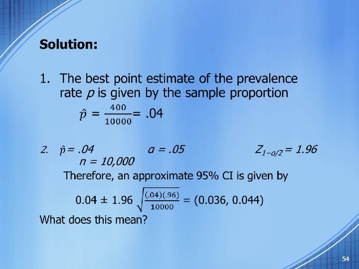
Estimation of a population proportion P • We are frequently interested in estimating the proportion of a population with a characteristic of interest, such as: • the proportion of smokers • the proportion of cancer patients who survive at least 5 years • the proportion of new HIV patients who are female 47

§ The population of interest has a certain characteristics that appears with a certain proportion p. This proportion is a quantity that we usually don’t know, but we would like to estimate it. Since it is a characteristic of the population, we call it a parameter. § To estimate p we draw a representative sample of size n from the population and count the number of individuals (X) in the sample with the characteristic we are looking for. This gives us the estimate X/n. 48

Point estimation of P § This estimate, = X/n, is called the sampling proportion and it is denoted by 49

Sampling Distribution of Proportion • You learned that a binomial can be approximated by the normal distribution if np 5 and nq 5. • Provided we have a large enough sample size, all the possible sample proportions will be approximately normally distributed with: 50

Confidence Interval for the Population Proportion An approximate 100% × (1 − α) CI for the binomial parameter p based on the normal approximation to the binomial distribution is given by: 51

52

Example • Suppose we are interested in estimating the prevalence rate of breast cancer among 50 - to 54 year-old women whose mothers have had breast cancer. Suppose that in a random sample of 10, 000 such women, 400 are found to have had breast cancer at some point in their lives. 1. Estimate the prevalence of breast cancer among 50 - to 54 -year-old women whose mothers have had breast cancer. 2. Derive a 95% CI for the prevalence rate of breast cancer among 50 - to 54 -year-old women. 53

Determining Sample Size For estimating the Mean For estimating the Proportion

Sampling Error • The required sample size can be found to reach a desired margin of error (e) with a specified level of confidence (1 - ) • The margin of error is also called sampling error – the amount of imprecision in the estimate of the population parameter – the amount added and subtracted to the point estimate to form the confidence interval

Determining Sample Size for Estimating the Mean Now solve for n to get

Determining Sample Size (continued) • To determine the required sample size for the mean, you must know: – The desired level of confidence (1 - ), which determines the critical value, Zα/2 – The acceptable sampling error, e – The standard deviation, σ

Example If = 45, what sample size is needed to estimate the mean within ± 5 with 90% confidence? So the required sample size is n = 220 (Always round up)

If σ is unknown • If unknown, σ can be estimated when using the required sample size formula – Use a value for σ that is expected to be at least as large as the true σ – Select a pilot sample and estimate σ with the sample standard deviation, S

Determining Sample Size for Estimating the Proportion Now solve for n to get

Determining Sample Size (continued) • To determine the required sample size for the proportion, you must know: – The desired level of confidence (1 - ), which determines the critical value, Zα/2 – The acceptable sampling error, e – The true proportion of events of interest, π • π can be estimated with a pilot sample if necessary (or conservatively use 0. 5 as an estimate of π)

Example How large a sample would be necessary to estimate the true proportion of defectives in a large population within ± 3%, with 95% confidence? (Assume a pilot sample yields p = 0. 12)

(continued) Example Solution: For 95% confidence, use Zα/2 = 1. 96 e = 0. 03 p = 0. 12, so use this to estimate π So use n = 451

65

Introduction • Researchers often have preconceived ideas about what the values of these parameters might be and wish to test whether the data conform to these ideas. • Used to investigate the validity of a claim about the value of a population characteristic. • For example: 1. The hospital administrator may want to test the hypothesis that the average length of stay of patients admitted to the hospital is 5 days! 2. Suppose we want to test the hypothesis that mothers with low socioeconomic status (SES) deliver babies whose birth weights are lower than “normal. ” 66

• Hypothesis testing is widely used in medicine, dentistry, health care, biology and other fields as a means to draw conclusions about the nature of populations. • Why is hypothesis testing so important? Hypothesis testing provides an objective framework for making decisions using probabilistic methods, rather than relying on subjective impressions. Hypothesis testing is to provide information in helping to make decisions. 67

General Concepts • A hypothesis is a statement about one or more populations. There are research hypotheses and statistical hypotheses. • A research hypothesis is the supposition or conjecture that motivates the research. • Statistical hypotheses are stated in such a way that they may be evaluated by appropriate statistical techniques 68

Elements of a statistical hypothesis test – Null hypothesis (H 0): Statement regarding the value(s) of unknown parameter(s). It is the hypothesis to be tested. – Alternative hypothesis (H 1): Statement contradictory to the null hypothesis. It is a statement of what we believe is true if our sample data cause us to reject the null hypothesis. – Test statistic - Quantity based on sample data and null hypothesis used to test between null and alternative hypotheses – Rejection region - Values of the test statistic for which we reject the null in favor of the alternative hypothesis 69

4 possible outcomes in hypothesis testing Truth Decision H 0 H 1 Accept H 0 is true and H 0 is accepted H 1 is true and H 0 is accepted Correct decision Type II error (β) Reject H 0 is true and H 0 is rejected Type І error (α) H 1 is true and H 0 is rejected Correct decision • The probability of a type I error is the probability of rejecting the null hypothesis when H 0 is true, denoted by α and is commonly referred to as the significance level of a test. • The probability of a type II error is the probability of accepting the null hypothesis when H 1 is true, and usually denoted by β. 70

• The general aim in hypothesis testing is to use statistical tests that make α and β as small as possible. • This goal requires compromise because making α small will increase β. • Our general strategy is to fix α at some specific level (for example, . 10, . 05, . 01, . . . ) and to use the test that minimizes β or, equivalently, maximizes the power. 71

One-Sample Inferences 72

One-Sample Test for the Mean of a Normal Distribution One-Sided Tests • Hypothesis: – Null Hypothesis H 0 : μ = μ 0 – Alternative hypothesis H 1: μ < μ 0 or H 1 : μ > μ 0 • Identify level of significance: – is a predetermined value (e. g. , =. 05) 73

• Test statistic: – If is known, or if sample size is large – If is unknown, or if sample size is small 74

• Critical Value: the rejection region 75

Conclusion: • Left-tailed Test: – Reject H 0 if Z < Z 1 -α – Reject H 0 if t < tn-1, α (when use Z - test) (when use T - test) • Right-tailed Test – Reject H 0 if Z > Z 1 -α – Reject H 0 if t > t 1 -α, n-1 (when use Z - test) (when use T - test) • An Alternative Decision Rule using the p - value Definition 76

P-Value • The P-value (or p-value or probability value) is the probability of getting a value of the test statistic that is at least as extreme as the one representing the sample data, assuming that the null hypothesis is true. • The p-value is defined as the smallest value of α for which the null hypothesis can be rejected 77

• If the p-value is less than or equal to , we reject the null hypothesis (p ≤ ) • If the p-value is greater than , we do not reject the null hypothesis (p > ) 78

Two-Sided Tests • A two-tailed test is a test in which the values of the parameter being studied (in this case μ) under the alternative hypothesis are allowed to be either greater than or less than the values of the parameter under the null hypothesis (μ 0). • To test the hypothesis H 0 : μ = μ 0 H 1 : μ ≠ μ 0 79

• Using the Test statistic: – If is known, or if sample size is large – If is unknown, or if sample size is small 80

• Decision Rule: – Reject H 0 if Z >Z 1 -α/2 or Z< - Z 1 -α/2 (when use Z - test) – Reject H 0 if T > t 1 -α/2, n-1 or t < - t 1 -α/2, n-1 (when use T- test) Values that differ significantly from H 0 81

Example 1 • Among 157 Saudi men , the mean systolic blood pressure was 146 mm Hg with a standard deviation of 27. We wish to know if on the basis of these data, we may conclude that the mean systolic blood pressure for a population of Saudi is greater than 140. Use =0. 01. 82

• = 2. 78 83

• Decision Rule: – we reject H 0 if Z > Z 1 -α – Z 0. 99= 2. 33 from table Z • Decision: – Since 2. 78 > 2. 33. then we reject H 0 What is our final conclusion? 84

Example 2 • The following are the systolic blood pressures of 12 patients undergoing drug therapy for hypertension: 183, 152, 178, 157, 194, 163, 144, 114, 178, 152, 118, 158 Can we conclude on the basis of these data that the population mean of SBP is less than 165? Use =0. 05. Use SPSS to do this! Here is unknown and sample size is small! 85

Solution: State your hypotheses: H 0 : μ = 165 H 1: μ < 165 Analyze Means Compare One-Sample T Test Select the variable Set the test value μ 0 86

The results of this test Sample mean Sample standard dev. T test statistic P-value (two-tailed) Mean from null hyp. Here, the two-tailed P-value is 0. 315. Since we are conducting a onetailed test, the P-value is 0. 315/2 = 0. 1575. Since p-value > 0. 05. Then we fail to reject H 0. 87

Using Excel 88

Excel Output Mean Variance Observations Hypothesized Mean Difference df t Stat P(T<=t) one-tail t Critical one-tail P(T<=t) two-tail t Critical two-tail SBP 157. 58 595. 36 12 165 11 -1. 05 0. 16 1. 80 0. 31 2. 20 89

One-Sample Test for the Population Proportion P (binomial distribution) • Recall that: The sampling distribution of a sample proportion is approximately normal (normal approximation of a binomial distribution) when the sample size is large enough. • Thus, we can easily test the null hypothesis: H 0 : p = p 0 • Alternative Hypotheses: 90

• Test Statistic: • Decision Rule: If H 1: P ≠ P 0 Reject H 0 if Z > Z 1 -α/2 or Z < - Z 1 -α/2 If H 1: P > P 0 Reject H 0 if Z > Z 1 -α If H 1: P < P 0 Reject H 0 if Z < - Z 1 -α 91

Example • Historically, one in five kidney cancer patients survive 5 years past diagnosis, i. e. 20%. • An oncologist using an experimental therapy treats n = 40 kidney cancer patients and 16 of them survive at least 5 years. • Is there evidence that patients receiving the experimental therapy have a higher 5 -year survival rate? 92

p = the proportion of kidney cancer patients receiving the experimental therapy that survive at least 5 years. Determine test criteria Choose =. 05 (may want to consider smaller? ) Use large sample test since: np = (40)(. 20) = 8 > 5 and n(1 -p) = (40)(. 80) = 32 > 5 93

Conclusion: Z 1 -α = Z 0. 95 = 1. 64 Since Z > Z 1 -α Reject H 0 What is our final conclusion? 0 1. 64 z 94

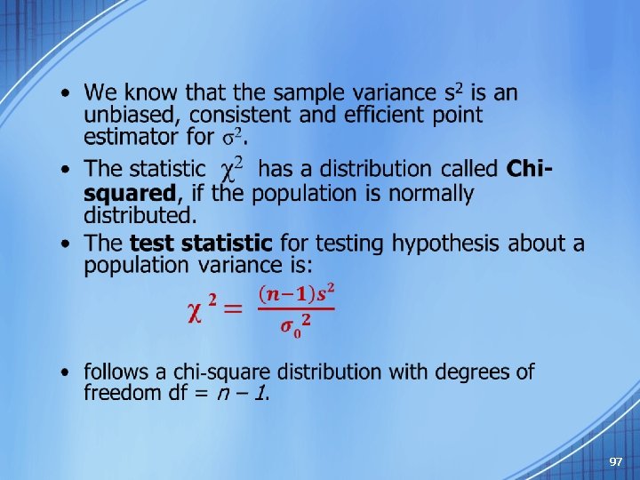
One-Sample Test for Variance and Standard Deviation • Why test variance ? – In real life, things vary. Even under strictest conditions, results will be different between one another. This causes variances. – When we get a sample of data, apart from testing on the mean to find if it is reasonable, we also test the variance to see whether certain factor has caused greater or smaller variation among the data. – In nature, variation exists. Even identical twins have some differences. This makes life interesting! 95

• Sometimes we are interested in making inference about the variability of processes. • Examples: – The consistency of a production process for quality control purposes. – Investors use variance as a measure of risk. • To draw inference about variability, the parameter of interest is σ2. 96

• If we want to test the following hypothesis: • reject H 0 if: χ2 < χ2 n-1, α/2 χ2 > χ2 n-1, 1 - α/2 or α/2 χ2 n-1, 1 - α/2 χ2 98

Example • A local balloon company claims that the variance for the time one of its helium balloons will stay afloat is 5 seconds. • A disgruntled customer wants to test this claim. • She randomly selects 23 customers and finds that the variance of the sample is 4. 5 seconds. • At = 0. 05, does she have enough evidence to reject the company’s claim? 99

• Hypothesis to be tested: H 0 : 2 = 5 (Claim) H 1 : 2 5 • Test statistic: Fail to reject H 0. Conclusion: At = 0. 05, there is not enough evidence to reject the claim that the variance of the float time is 5 seconds. X 2 10. 982 36. 781 From Chi-square Table 100

Two-Sample Inferences 101

Hypothesis Testing: Two-Sample Inference • A more frequently encountered situation is the two-sample hypothesis-testing problem. • In a two-sample hypothesis-testing problem, the underlying parameters of two different populations, neither of whose values is assumed known, are compared. • Distinguish between Independent and Dependent Sampling. 102

• Two samples are said to be independent when the data points in one sample are unrelated to the data points in the second sample. • Two samples are said to be Dependent (paired) when each data point in the first sample is matched and is related to a unique data point in the second sample. • Dependent samples are often referred to as matched-pairs samples. 103

Inference about Two Population Means The Paired t - test • Statistical inference methods on matched-pairs data use the same methods as inference on a single population mean with unknown, except that the differences are analyzed. di = xi 2 − xi 1 • The hypothesis testing problem can thus be considered a one-sample t test based on the differences (di ). 104

• To test hypotheses regarding the mean difference of matched-pairs data, the following must be satisfied: 1. the sample is obtained using simple random sampling 2. the sample data are matched pairs, 3. the differences are normally distributed with no outliers or the sample size, n, is large (n ≥ 30). 105

Step 1: • Determine the null and alternative hypotheses. The hypotheses can be structured in one of three ways, where μd is the population mean difference of the matched-pairs data. 106

Step 2: • Select a level of significance, , based on the seriousness of making a Type I error. Step 3: • Compute the test statistic which approximately follows Student’ t-distribution with n-1 degrees of freedom • The values of and sd are the mean and standard deviation of the differenced data. 107

Step 4: • Use Table t to determine the critical value using n 1 degrees of freedom. Step 5: • Compare the critical value with the test statistic: • If P-value < , reject the null hypothesis. 108

Example: Hypertension • Let’s say we are interested in the relationship between oral contraceptive (OC) use and blood pressure in women. • Identify a group of non-pregnant, premenopausal women of childbearing age (16 – 49 years) who are not currently OC users, and measure their blood pressure, which will be called the baseline blood pressure. • Rescreen these women 1 year later to ascertain a subgroup who have remained non-pregnant throughout the year and have become OC users. This subgroup is the study population. 109

• Measure the blood pressure of the study population at the follow-up visit. • Compare the baseline and follow-up blood pressure of the women in the study population to determine the difference between blood pressure levels of women when they were using the pill at follow-up and when they were not using the pill at baseline. • Assume that the SBP of the ith woman is normally distributed at baseline with mean μi and variance σ2 and at follow-up with mean μi + d and variance σ2. 110

• If d = 0, then there is no difference between mean baseline and follow-up SBP. If d > 0, then using OC pills is associate with a raised mean SBP. If d < 0, then using OC pills is associated with a lowered mean SBP. • We want to test the hypothesis: H 0: μd = 0 vs. H 1: μd ≠ 0. • How should we do this? 111

Solution: • Using SPSS – After Importing your dataset, and providing names to variables, click on: – ANALYZE COMPARE MEANS PAIRED SAMPLES T-TEST – For PAIRED VARIABLES, Select the two dependent (response) variables (the analysis will be based on first variable minus second variable) 112

sd p-value Since the exact two-sided p-value =. 009 < 0. 05, we reject the null hypothesis. Therefore, we can conclude that starting OC use is associated with a significant change in blood pressure. 113

• A two-sided 100% × (1 − α) CI for the true mean difference (μd) between two paired samples is given by: Compute a 95% CI for the true increase in mean SBP after starting OCs. (1. 53, 8. 07) Note that the conclusion from the hypothesis test and the confidence interval are the same! 114

Using Excel 115

Excel Output: OC 120. 4 174. 933 10 0. 955 0 9 3. 325 0. 004 1. 833 0. 009 2. 262 NONOC 115. 6 106. 267 10 Mean Variance Observations Pearson Correlation Hypothesized Mean Difference df t Stat P(T<=t) one-tail t Critical one-tail P(T<=t) two-tail t Critical two-tail Since the p-value =. 009 < 0. 05, we reject the null hypothesis. Therefore, we can conclude that starting OC use is associated with a significant change in blood pressure. 116

Two-Sample T-Test for Independent Samples Equal Variances: • The independent samples t-test is probably the single most widely used test in statistics. • It is used to compare differences between separate groups. • We want to test the hypothesis: H 0: μ 1 = μ 2 vs. H 1: μ 1 ≠ μ 2 or μ 1 > μ 2 or μ 1 < μ 2 • Sometimes we will be willing to assume that the variance in the two groups is equal: 117

• If we know this variance, we can use the z-statistic • Often we have to estimate 2 with the sample variance from each of the samples, • Since we have two estimates of one quantity, we pool the two estimates. 118

• The average of estimate of σ2 : and could simply be used as the • The t-statistic based on the pooled variance is very similar to the z-statistic as always: • The t-statistic has a t-distribution with freedom degrees of 119

Constructing a (1 - )100 % Confidence Interval for the Difference of Two Means: equal variances • If the two populations are normally distributed or the sample sizes are sufficiently large (n 1≥ 30 and n 2≥ 30), and a (1 - )100 % confidence interval about 1 - 2 is given by: [ ] 120

Unequal variance • Often, we are unwilling to assume that the variances are equal! • The test statistic as: • The distribution of this statistic is difficult to derive and we approximate the distribution using a t-distribution with n degrees of freedom • This is called the Satterthwaite or Welch approximation 121

Constructing a (1 - )100 % Confidence Interval for the Difference of Two Means (Unequal variance) • If the two populations are normally distributed or the sample sizes are sufficiently large (n 1≥ 30 and n 2≥ 30), a (1 - )100 % confidence interval about 1 - 2 is given by: [ ] 122

Equality of variance • Since we can never be sure if the variances are equal, could we test if they are equal? • Of course we can!! – But, remember there is error in every statistical test. – Sometimes it is just preferred to use the unequal variance unless there is a good reason. • Test: H 0: 12 = 22 vs. H 1: 12 ≠ 22 with significance level . • To test this hypothesis, we use the sample variances: 123

Testing for the Equality of Two Variances • One way to test if the two variances are equal is to check if the ratio is equal to 1 (H 0: ratio=1) • Under the null, the ratio simplifies to • The ratio of 2 chi-square random variables has an F-distribution. • The F-distribution is defined by the numerator and denominator degrees of freedom. • Here we have an F-distribution with n 1 -1 and n 21 degrees of freedom 124

Strategy for testing for the equality of means in two independent, normally distributed samples Perform F-test for the equality of two variances t n a ic ≤ α f i n e g i S alu P-v No t P-v signi f alu e > icant α Perform t-test assuming unequal variances Perform t-test assuming equal variances 125

Example • Use hypothesis testing for Hospital-stay data in Table 2. 11 (page 33 in the book) to answer (2. 3). • Use SPSS to do the analysis! 2. 3: It is of clinical interest to know if the duration of hospitalization is affected by whether a patient has received antibiotics. That is to compare the mean duration of hospitalization between antibiotic users and non -antibiotic users. 126

Solution H 0 : μ 1 = μ 2 H 1 : μ 1 ≠ μ 2 μ 1 the mean duration of hospitalization for antibiotic users μ 2 the mean duration of hospitalization for non-antibiotic users 127

SPSS output H 0: 12 = 22 vs. H 1: 12 ≠ 22 H 0 : μ 1 = μ 2 vs. H 1 : μ 1 ≠ μ 2 Since p-value =0. 075 > 0. 05, then H 0 is NOT rejected Since p-value =0. 106 > 0. 05, then H 0 is NOT rejected 128

Using Excel 129

Excel Output: Mean Variance Observations Pooled Variance Hypothesized Mean Difference df t Stat P(T<=t) one-tail t Critical one-tail P(T<=t) two-tail t Critical two-tail DOHSANTI 11. 571 77. 619 7 30. 355 0 23 1. 682 0. 053 1. 714 0. 106 2. 069 DOHSNOANTI 7. 444 13. 673 18 Since p-value =0. 106 > 0. 05, then H 0 is NOT rejected, and conclude that the duration of hospitalization is affected by whether a patient has received antibiotics 130

Conclusion • First step in comparing the two means is to perform the F -test for the equality of two variances in order to decide whether to use the t-test with equal or unequal variances. • The p -value = 0. 075 > 0. 05. Thus the variances DO NOT differ significantly, and a two-sample t-test with equal variances should be used. • Therefore, refer to the Equal Variance row, where the tstatistic is 1. 68 with degrees of freedom d’(df). = 23. • The corresponding two-tailed p-value = 0. 106 > 0. 05. • Thus no significant difference exists between the mean duration of hospitalization in these two groups. 131

The Treatment of Outliers • Outliers can have an important impact on the conclusions of a study. • It is important to definitely identify outliers and either: 1. Exclude them! ( NOT recommended) or 2. Perform alternative analyses with and without the outliers present. 3. Use a method of analysis that minimizes their effect on the overall results. 132

Box-Plot 133

Inference about Two Population Proportions • Testing hypothesis about two population proportion (P 1 , P 2 ) is carried out in much the same way as for difference between two means when condition is necessary for using normal curve are met. 134

• We have the following: Data: sample size (n 1 ﻭ n 2), - Characteristic in two samples (x 1 , x 2), - sample proportions - Pooled proportion 135

Assumption: Two populations are independent. Hypotheses: Determine the null and alternative hypotheses. The hypotheses can be structured in one of three ways Select a level of significance α, based on the seriousness of making a Type I error. 136

• Compute the test statistic: • Decision Rule: – Compare the critical value with the test statistic: – Or, if P-value < α , reject the null hypothesis 137

Example • An economist believes that the percentage of urban households with Internet access is greater than the percentage of rural households with Internet access. • He obtains a random sample of 800 urban households and finds that 338 of them have Internet access. He obtains another random sample of 750 rural households and finds that 292 of them have Internet access. • Test the economist’s claim at the =0. 05 level of significance. 138

Solution: • The samples are simple random samples that were obtained independently. x 1=338, n 1=800, x 2=292 and n 2=750, so • We want to determine whether the percentage of urban households with Internet access is greater than the percentage of rural households with Internet access. 139

• So, we test the hypothesis: H 0 : p 1 = p 2 versus H 1 : p 1 > p 2 or, equivalently, H 0: p 1 - p 2=0 versus H 1 : p 1 - p 2 > 0 The level of significance is = 0. 05 140

The pooled estimate: The test statistic is: 141

• This is a right-tailed test with =0. 05 The critical value is Z 0. 05=1. 645 Since the test statistic, z 0=1. 33 is less than the critical value z. 05=1. 645, Then we fail to reject the null hypothesis. Conclusion: The percentage of urban households with Internet access is the same as the percentage of rural households with Internet access. 142

Constructing a (1 - )100% Confidence Interval for the Difference between Two Population Proportions • To construct a (1 - ) 100% confidence interval for the difference between two population proportions: 143

The Relationship Between Hypothesis Testing and Confidence Intervals (Two-Sided Case) • Suppose we are testing H 0: μ = μ 0 vs. H 1 : μ ≠ μ 0 • H 0 is rejected with a two-sided level test if and only if the two-sided 100% (1 − ) CI for μ does not contain μ 0 • H 0 is accepted with a two-sided level test if and only if the two-sided 100% (1 − ) CI for μ does contain μ 0 144

Is the Population Normal? Yes No Is n ≥ 30 ? No Use nonparametrics test Is Yes Use z-test No Use t-test σ known? Yes Use z-test 145