Inference Inference calculating some useful quantity from a

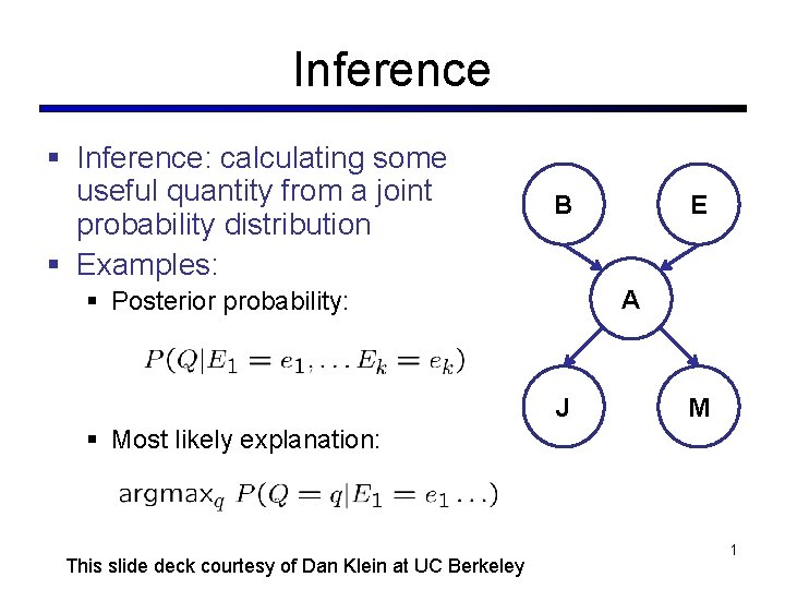
Inference § Inference: calculating some useful quantity from a joint probability distribution § Examples: B E A § Posterior probability: J M § Most likely explanation: This slide deck courtesy of Dan Klein at UC Berkeley 1

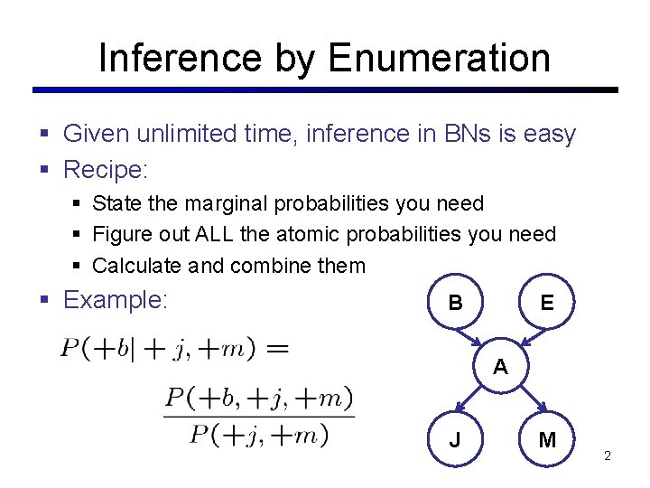
Inference by Enumeration § Given unlimited time, inference in BNs is easy § Recipe: § State the marginal probabilities you need § Figure out ALL the atomic probabilities you need § Calculate and combine them § Example: B E A J M 2

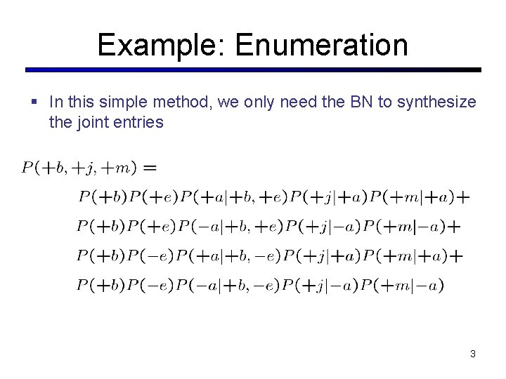
Example: Enumeration § In this simple method, we only need the BN to synthesize the joint entries 3

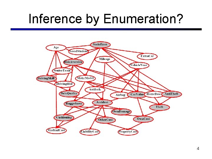
Inference by Enumeration? 4

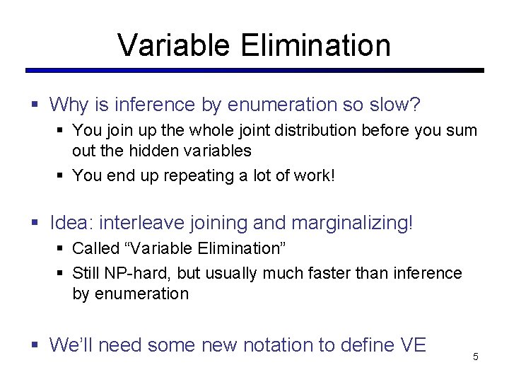
Variable Elimination § Why is inference by enumeration so slow? § You join up the whole joint distribution before you sum out the hidden variables § You end up repeating a lot of work! § Idea: interleave joining and marginalizing! § Called “Variable Elimination” § Still NP-hard, but usually much faster than inference by enumeration § We’ll need some new notation to define VE 5

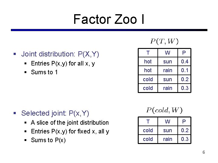
Factor Zoo I § Joint distribution: P(X, Y) § Entries P(x, y) for all x, y § Sums to 1 T W P hot sun 0. 4 hot rain 0. 1 cold sun 0. 2 cold rain 0. 3 T W P cold sun 0. 2 cold rain 0. 3 § Selected joint: P(x, Y) § A slice of the joint distribution § Entries P(x, y) for fixed x, all y § Sums to P(x) 6

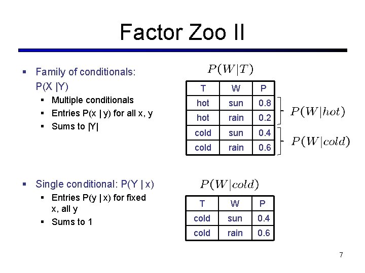
Factor Zoo II § Family of conditionals: P(X |Y) § Multiple conditionals § Entries P(x | y) for all x, y § Sums to |Y| T W P hot sun 0. 8 hot rain 0. 2 cold sun 0. 4 cold rain 0. 6 T W P cold sun 0. 4 cold rain 0. 6 § Single conditional: P(Y | x) § Entries P(y | x) for fixed x, all y § Sums to 1 7

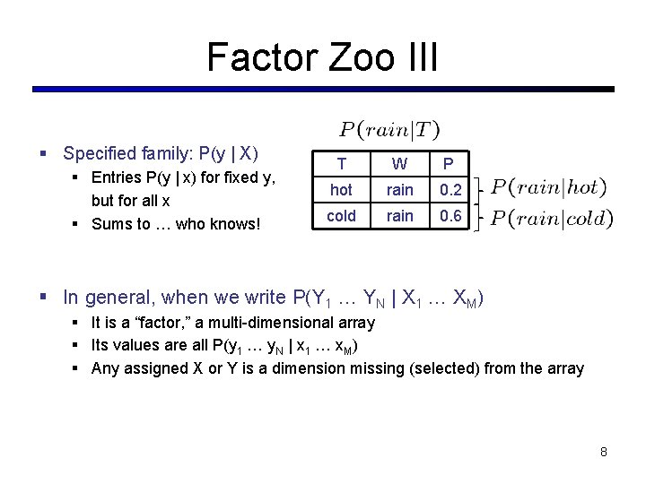
Factor Zoo III § Specified family: P(y | X) § Entries P(y | x) for fixed y, but for all x § Sums to … who knows! T W P hot rain 0. 2 cold rain 0. 6 § In general, when we write P(Y 1 … YN | X 1 … XM) § It is a “factor, ” a multi-dimensional array § Its values are all P(y 1 … y. N | x 1 … x. M) § Any assigned X or Y is a dimension missing (selected) from the array 8

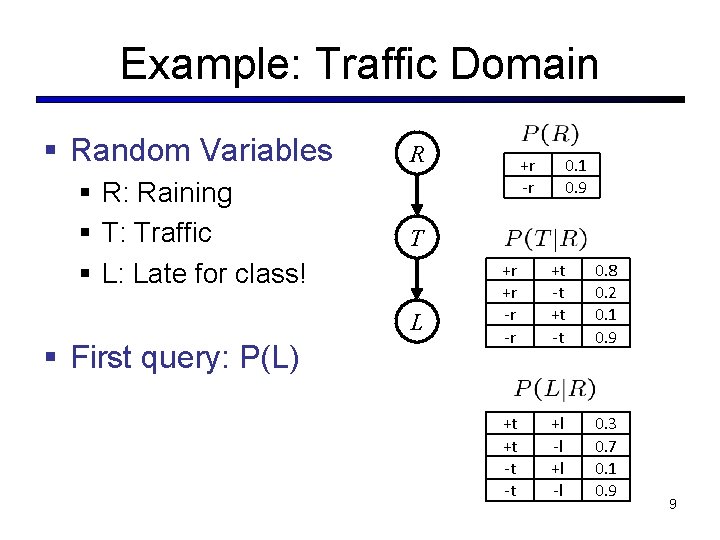
Example: Traffic Domain § Random Variables R § R: Raining § T: Traffic § L: Late for class! T L § First query: P(L) +r -r 0. 1 0. 9 +r +r -r -r +t -t 0. 8 0. 2 0. 1 0. 9 +t +t -t -t +l -l 0. 3 0. 7 0. 1 0. 9 9

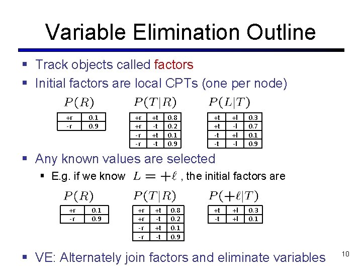
Variable Elimination Outline § Track objects called factors § Initial factors are local CPTs (one per node) +r -r 0. 1 0. 9 +r +r -r -r +t -t 0. 8 0. 2 0. 1 0. 9 +t +t -t -t +l -l 0. 3 0. 7 0. 1 0. 9 § Any known values are selected § E. g. if we know +r -r 0. 1 0. 9 , the initial factors are +r +r -r -r +t -t 0. 8 0. 2 0. 1 0. 9 +t -t +l +l 0. 3 0. 1 § VE: Alternately join factors and eliminate variables 10

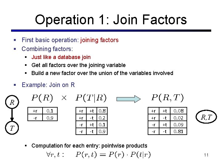
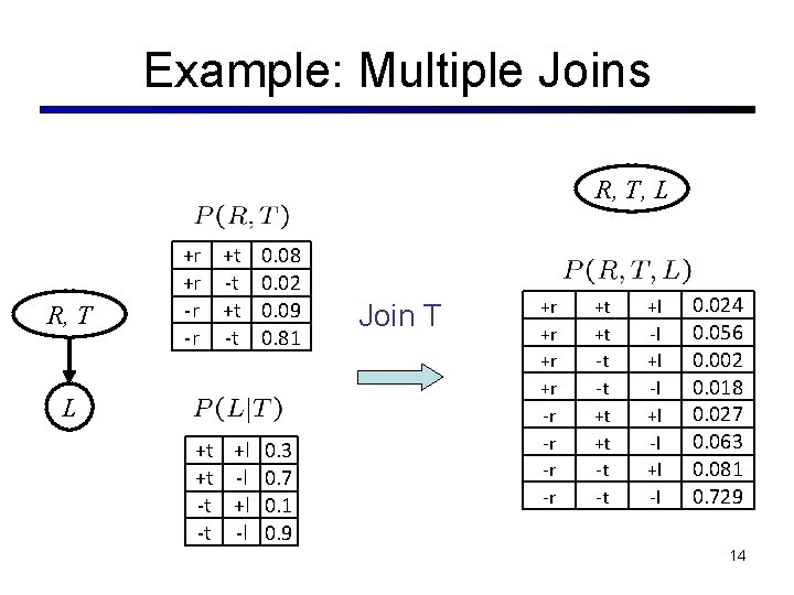
Operation 1: Join Factors § First basic operation: joining factors § Combining factors: § Just like a database join § Get all factors over the joining variable § Build a new factor over the union of the variables involved § Example: Join on R R +r -r T 0. 1 0. 9 +r +r -r -r +t -t 0. 8 0. 2 0. 1 0. 9 +r +r -r -r +t -t 0. 08 0. 02 0. 09 0. 81 R, T § Computation for each entry: pointwise products 11

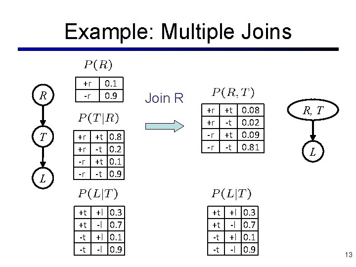
Example: Multiple Joins R T L +r -r +r +r -r -r 0. 1 0. 9 +t -t 0. 8 0. 2 0. 1 0. 9 +t +l 0. 3 +t -l 0. 7 -t +l 0. 1 -t -l 0. 9 Join R +r +t 0. 08 +r -t 0. 02 -r +t 0. 09 -r -t 0. 81 +t +l 0. 3 +t -l 0. 7 -t +l 0. 1 -t -l 0. 9 R, T L 13

Example: Multiple Joins R, T, L R, T +r +t 0. 08 +r -t 0. 02 -r +t 0. 09 -r -t 0. 81 L +t +l 0. 3 +t -l 0. 7 -t +l 0. 1 -t -l 0. 9 Join T +r +r -r -r +t +t -t -t +l -l 0. 024 0. 056 0. 002 0. 018 0. 027 0. 063 0. 081 0. 729 14

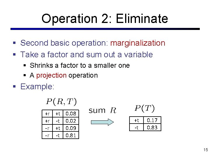
Operation 2: Eliminate § Second basic operation: marginalization § Take a factor and sum out a variable § Shrinks a factor to a smaller one § A projection operation § Example: +r +t 0. 08 +r -t 0. 02 -r +t 0. 09 -r -t 0. 81 +t -t 0. 17 0. 83 15

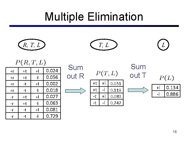
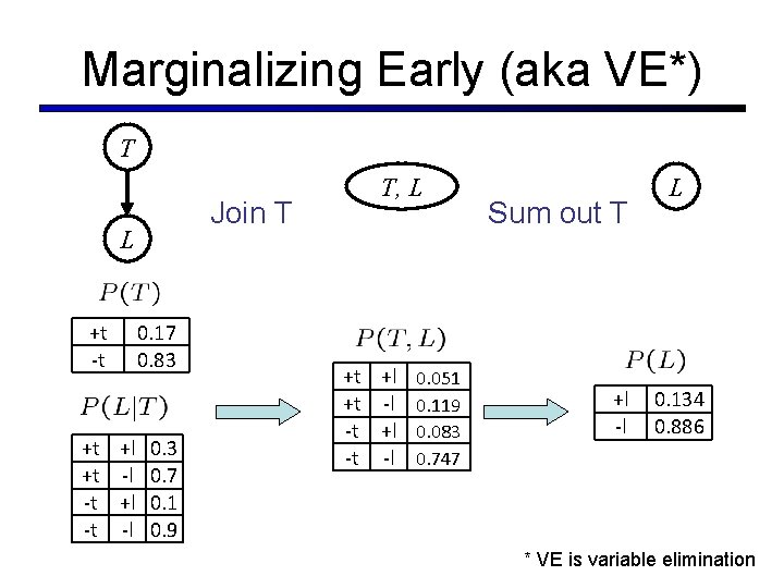
Multiple Elimination R, T, L +r +r -r -r +t +t -t -t +l -l T, L 0. 024 0. 056 0. 002 0. 018 0. 027 0. 063 0. 081 0. 729 Sum out R L Sum out T +t +l 0. 051 +t -l 0. 119 -t +l 0. 083 -t -l 0. 747 +l -l 0. 134 0. 886 16

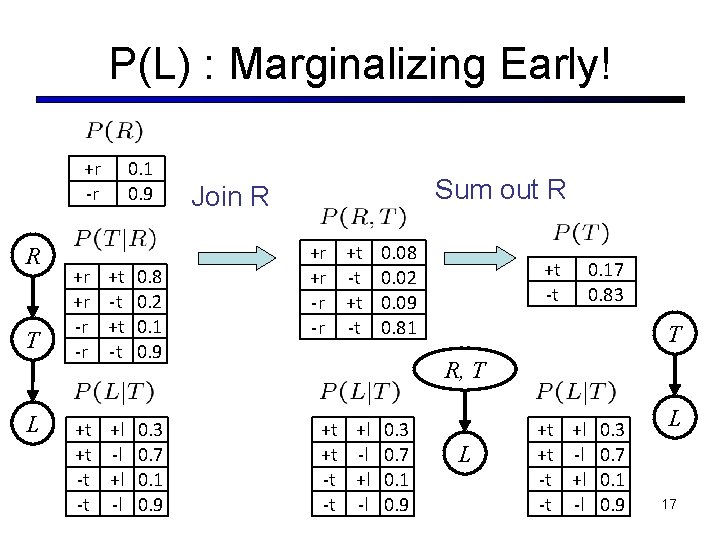
P(L) : Marginalizing Early! +r -r R T L +r +r -r -r 0. 1 0. 9 +t -t 0. 8 0. 2 0. 1 0. 9 +t +l 0. 3 +t -l 0. 7 -t +l 0. 1 -t -l 0. 9 Sum out R Join R +r +t 0. 08 +r -t 0. 02 -r +t 0. 09 -r -t 0. 81 +t -t 0. 17 0. 83 T R, T +t +l 0. 3 +t -l 0. 7 -t +l 0. 1 -t -l 0. 9 L 17

Marginalizing Early (aka VE*) T Join T L +t -t 0. 17 0. 83 +t +l 0. 3 +t -l 0. 7 -t +l 0. 1 -t -l 0. 9 T, L +t +l 0. 051 +t -l 0. 119 -t +l 0. 083 -t -l 0. 747 Sum out T +l -l L 0. 134 0. 886 * VE is variable elimination

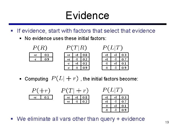
Evidence § If evidence, start with factors that select that evidence § No evidence uses these initial factors: +r -r 0. 1 0. 9 +r +r -r -r +t -t § Computing +r 0. 1 0. 8 0. 2 0. 1 0. 9 +t +t -t -t +l -l 0. 3 0. 7 0. 1 0. 9 , the initial factors become: +r +r +t -t 0. 8 0. 2 +t +t -t -t +l -l 0. 3 0. 7 0. 1 0. 9 § We eliminate all vars other than query + evidence 19

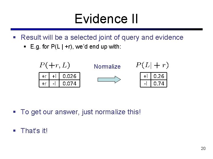
Evidence II § Result will be a selected joint of query and evidence § E. g. for P(L | +r), we’d end up with: Normalize +r +l +r -l 0. 026 0. 074 +l -l 0. 26 0. 74 § To get our answer, just normalize this! § That’s it! 20

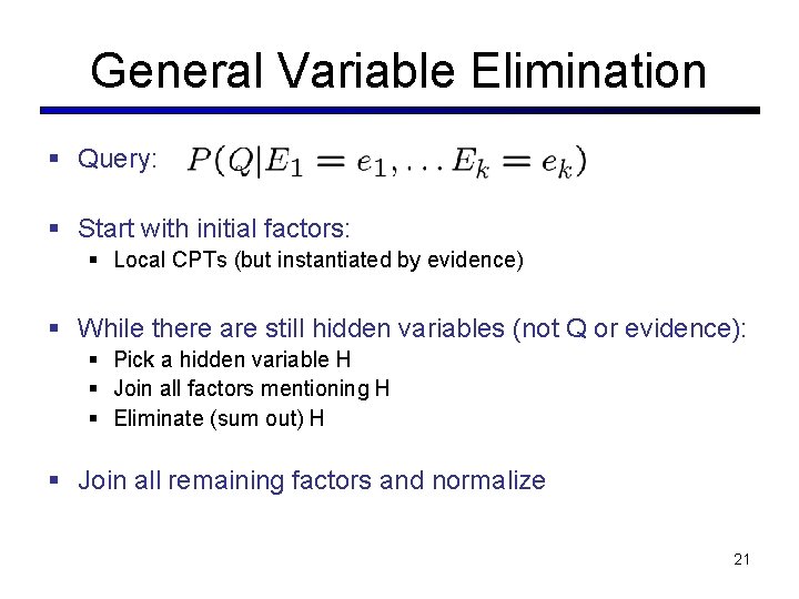
General Variable Elimination § Query: § Start with initial factors: § Local CPTs (but instantiated by evidence) § While there are still hidden variables (not Q or evidence): § Pick a hidden variable H § Join all factors mentioning H § Eliminate (sum out) H § Join all remaining factors and normalize 21

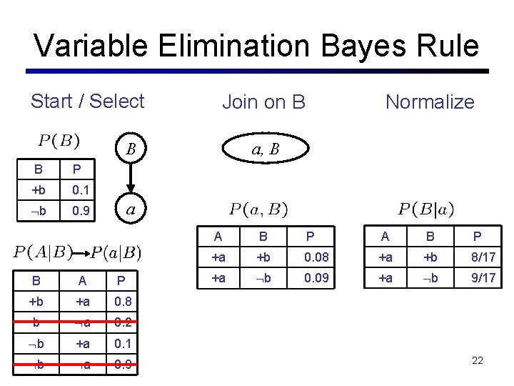
Variable Elimination Bayes Rule Start / Select Join on B B B P +b 0. 1 b 0. 9 Normalize a, B a B A P +b +a 0. 8 b a 0. 2 b +a 0. 1 b a 0. 9 A B P +a +b 0. 08 +a +b 8/17 +a b 0. 09 +a b 9/17 22

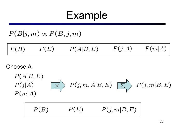
Example Choose A 23

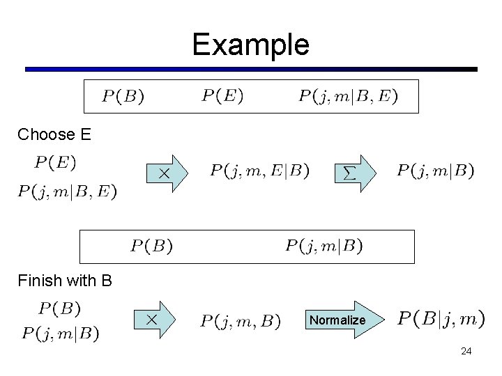
Example Choose E Finish with B Normalize 24

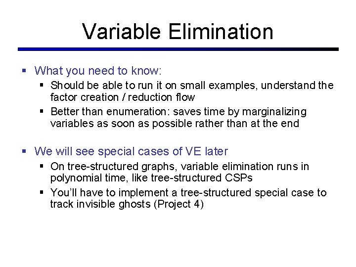
Variable Elimination § What you need to know: § Should be able to run it on small examples, understand the factor creation / reduction flow § Better than enumeration: saves time by marginalizing variables as soon as possible rather than at the end § We will see special cases of VE later § On tree-structured graphs, variable elimination runs in polynomial time, like tree-structured CSPs § You’ll have to implement a tree-structured special case to track invisible ghosts (Project 4)

26

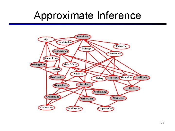
Approximate Inference 27

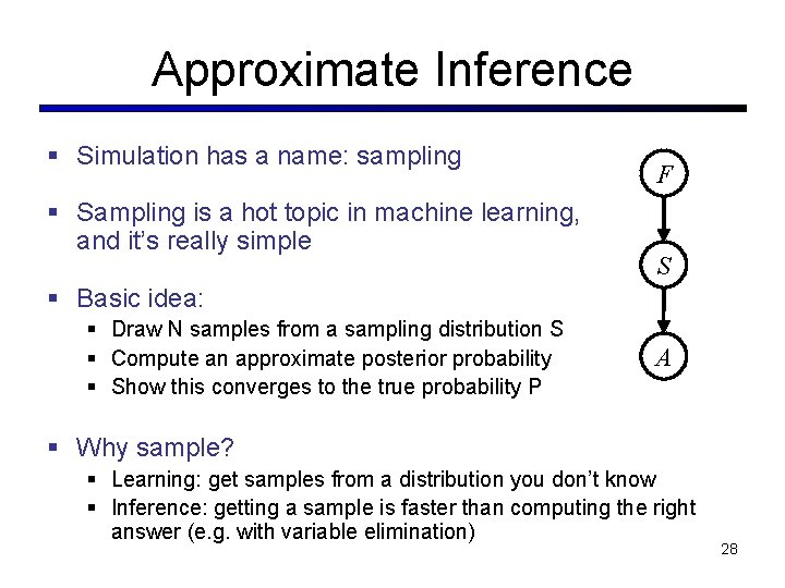
Approximate Inference § Simulation has a name: sampling § Sampling is a hot topic in machine learning, and it’s really simple F S § Basic idea: § Draw N samples from a sampling distribution S § Compute an approximate posterior probability § Show this converges to the true probability P A § Why sample? § Learning: get samples from a distribution you don’t know § Inference: getting a sample is faster than computing the right answer (e. g. with variable elimination) 28

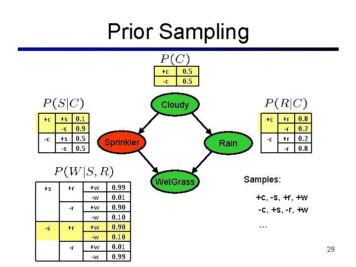
Prior Sampling +c -c 0. 5 Cloudy +c -c +s +s -s 0. 1 0. 9 0. 5 +r -r -s +r -r +c Sprinkler +w -w 0. 99 0. 01 0. 90 0. 10 0. 01 0. 99 Rain Wet. Grass -c +r -r 0. 8 0. 2 0. 8 Samples: +c, -s, +r, +w -c, +s, -r, +w … 29

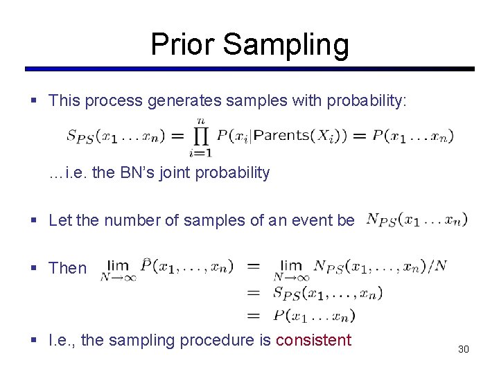
Prior Sampling § This process generates samples with probability: …i. e. the BN’s joint probability § Let the number of samples of an event be § Then § I. e. , the sampling procedure is consistent 30

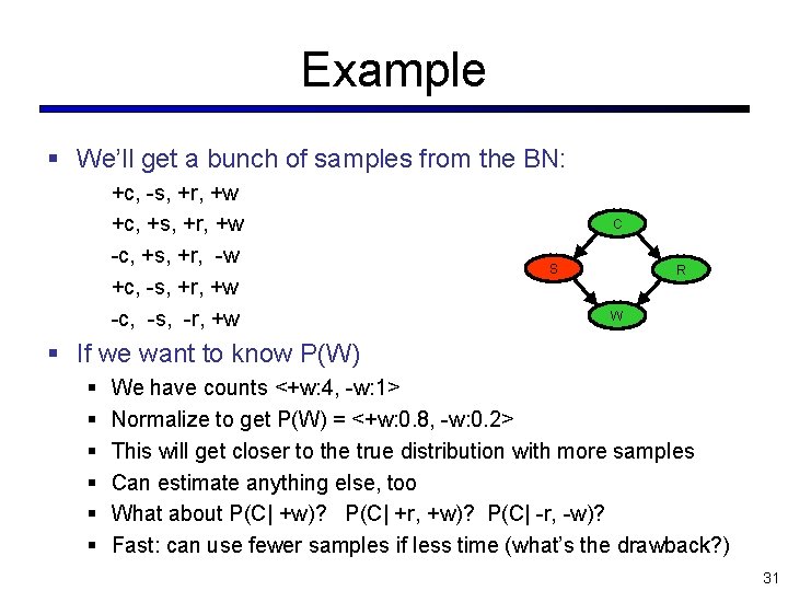
Example § We’ll get a bunch of samples from the BN: +c, -s, +r, +w +c, +s, +r, +w -c, +s, +r, -w +c, -s, +r, +w -c, -s, -r, +w Cloudy C Sprinkler S Rain R Wet. Grass W § If we want to know P(W) § § § We have counts <+w: 4, -w: 1> Normalize to get P(W) = <+w: 0. 8, -w: 0. 2> This will get closer to the true distribution with more samples Can estimate anything else, too What about P(C| +w)? P(C| +r, +w)? P(C| -r, -w)? Fast: can use fewer samples if less time (what’s the drawback? ) 31

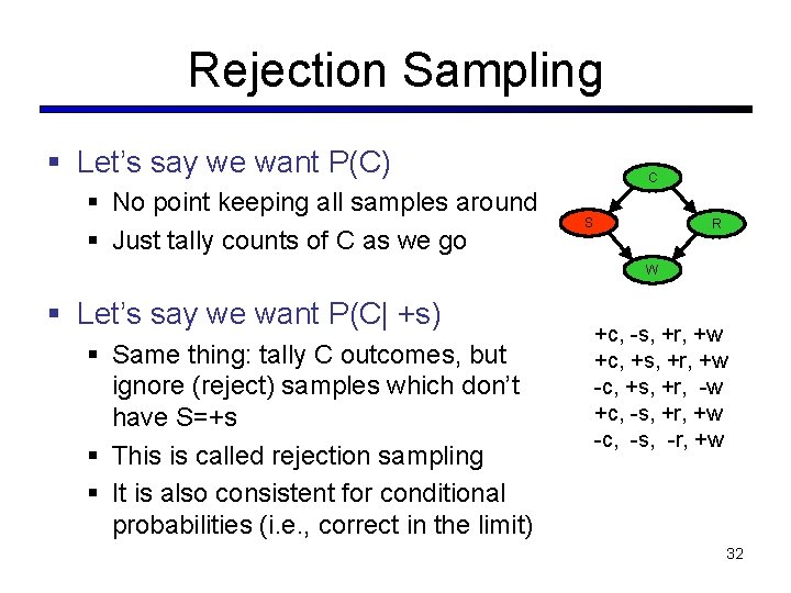
Rejection Sampling § Let’s say we want P(C) § No point keeping all samples around § Just tally counts of C as we go Cloudy C Sprinkler S Rain R Wet. Grass W § Let’s say we want P(C| +s) § Same thing: tally C outcomes, but ignore (reject) samples which don’t have S=+s § This is called rejection sampling § It is also consistent for conditional probabilities (i. e. , correct in the limit) +c, -s, +r, +w +c, +s, +r, +w -c, +s, +r, -w +c, -s, +r, +w -c, -s, -r, +w 32

Sampling Example § There are 2 cups. § The first contains 1 penny and 1 quarter § The second contains 2 quarters § Say I pick a cup uniformly at random, then pick a coin randomly from that cup. It's a quarter (yes!). What is the probability that the other coin in that cup is also a quarter?

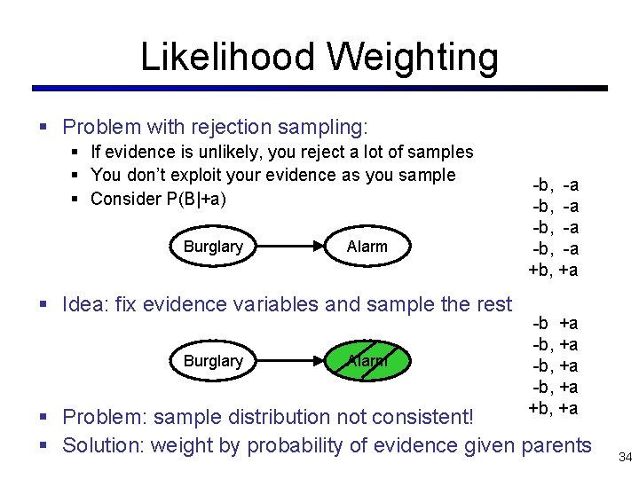
Likelihood Weighting § Problem with rejection sampling: § If evidence is unlikely, you reject a lot of samples § You don’t exploit your evidence as you sample § Consider P(B|+a) Burglary Alarm § Idea: fix evidence variables and sample the rest Burglary Alarm -b, -a +b, +a -b, +a +b, +a § Problem: sample distribution not consistent! § Solution: weight by probability of evidence given parents 34

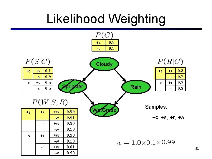
Likelihood Weighting +c -c 0. 5 Cloudy +c -c +s +s -s 0. 1 0. 9 0. 5 +r -r -s +r -r +c Sprinkler +w -w 0. 99 0. 01 0. 90 0. 10 0. 01 0. 99 Rain Wet. Grass -c +r -r 0. 8 0. 2 0. 8 Samples: +c, +s, +r, +w … 35

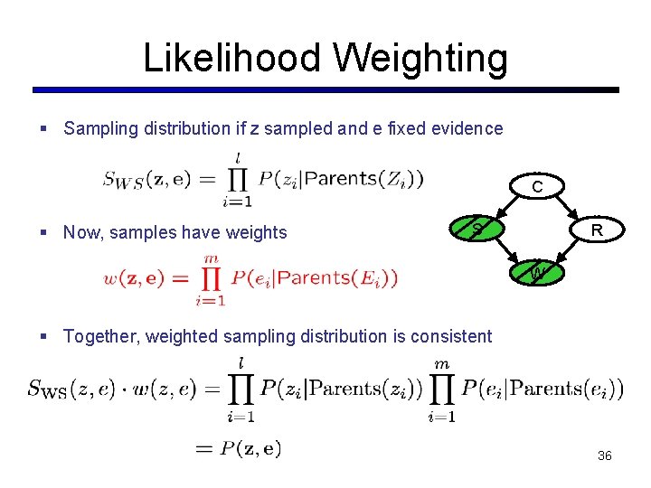
Likelihood Weighting § Sampling distribution if z sampled and e fixed evidence Cloudy C § Now, samples have weights S R W § Together, weighted sampling distribution is consistent 36

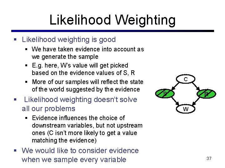
Likelihood Weighting § Likelihood weighting is good § We have taken evidence into account as we generate the sample § E. g. here, W’s value will get picked based on the evidence values of S, R § More of our samples will reflect the state of the world suggested by the evidence § Likelihood weighting doesn’t solve all our problems Cloudy C S Rain R W § Evidence influences the choice of downstream variables, but not upstream ones (C isn’t more likely to get a value matching the evidence) § We would like to consider evidence when we sample every variable 37

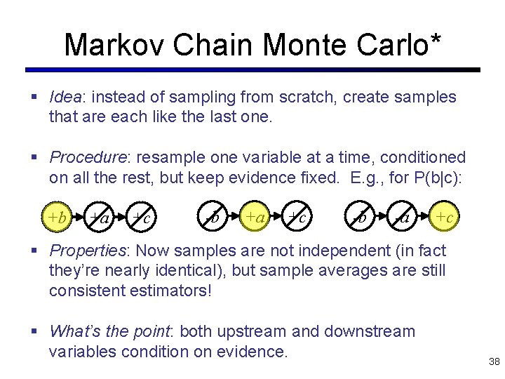
Markov Chain Monte Carlo* § Idea: instead of sampling from scratch, create samples that are each like the last one. § Procedure: resample one variable at a time, conditioned on all the rest, but keep evidence fixed. E. g. , for P(b|c): +b +a +c -b -a +c § Properties: Now samples are not independent (in fact they’re nearly identical), but sample averages are still consistent estimators! § What’s the point: both upstream and downstream variables condition on evidence. 38