Inference for Two Proportions Concepts in Statistics Inferences

Inference for Two Proportions Concepts in Statistics

Inferences about a Population Proportion • • Random samples vary. When we use a sample proportion to make an inference about a population proportion, there is uncertainty. Inference involves probability. Under certain conditions, we can model the variability in sample proportions with a normal curve. We use the normal curve to make probability-based decisions about population values. We can estimate a population proportion with a confidence interval. The confidence interval is an actual sample proportion with a margin of error. We state our confidence in the accuracy of these intervals using probability. We can test a hypothesis about a population proportion using an actual sample proportion. We base our conclusion on probability using a P-value. The P-value describes the strength of our evidence in rejecting a hypothesis about the population.

Steps in a Statistical Investigation Produce Data: Determine what to measure, then collect the data. Collect categorical data from two samples. In an observational study, we begin with two populations and randomly select a sample from each population. In an experiment, we randomly assign individuals to two treatments. Exploratory Data Analysis: Analyze and summarize the data. We are working with categorical data, so from each sample, we compute a sample proportion. To compare the two samples, we subtract the proportions. When we conduct inference in the next step, our goal is to determine if the actual difference in the sample proportions is significantly different from what we expect in random sampling.

Steps in a Statistical Investigation (continued) Draw a Conclusion: Use data, probability, and statistical inference to draw a conclusion about the populations. • We use simulation to observe the behavior of the differences in sample proportions when we randomly select many, many samples. We create the simulation to reflect a claim about the populations. Then develop a probability model to describe the shape, center, and spread of the sampling distribution. We are interested in the conditions that allow us to use a normal curve. • We use this model to determine when a given difference is unusual in a formal hypothesis test. • We also construct confidence intervals to estimate the difference between two population proportions. As before, we make a probability statement about our confidence in the accuracy of these intervals.

Distribution of Differences in Sample Proportions In the previous module, we learned to estimate and test hypotheses regarding the value of a single population proportion. In this module we want to develop tools comparing two unknown population proportions. The first step is to examine how random samples from the populations compare. In this investigation, we assume we know the population proportions in order to develop a model for the sampling distribution.

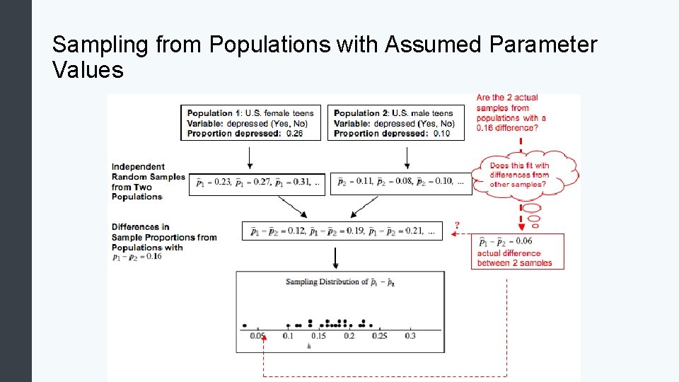
Sampling from Populations with Assumed Parameter Values

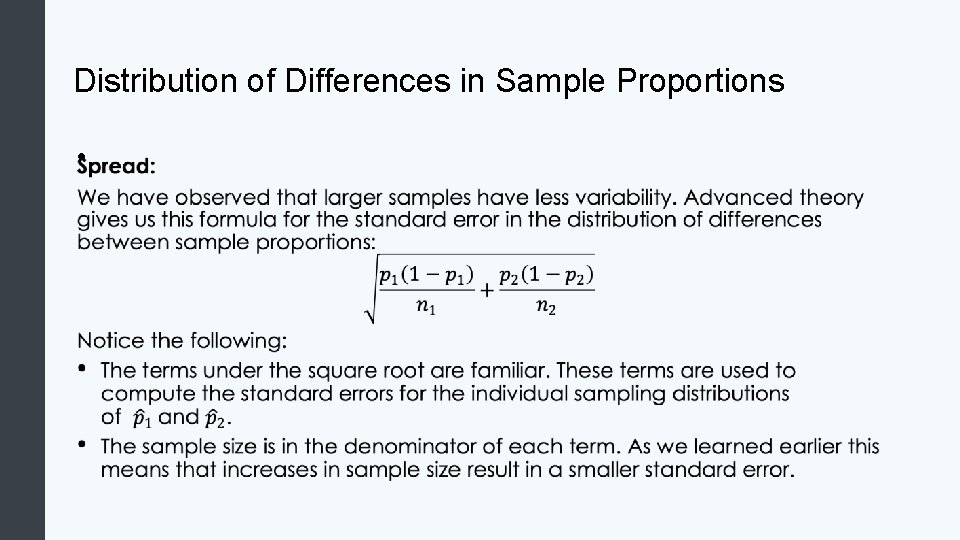
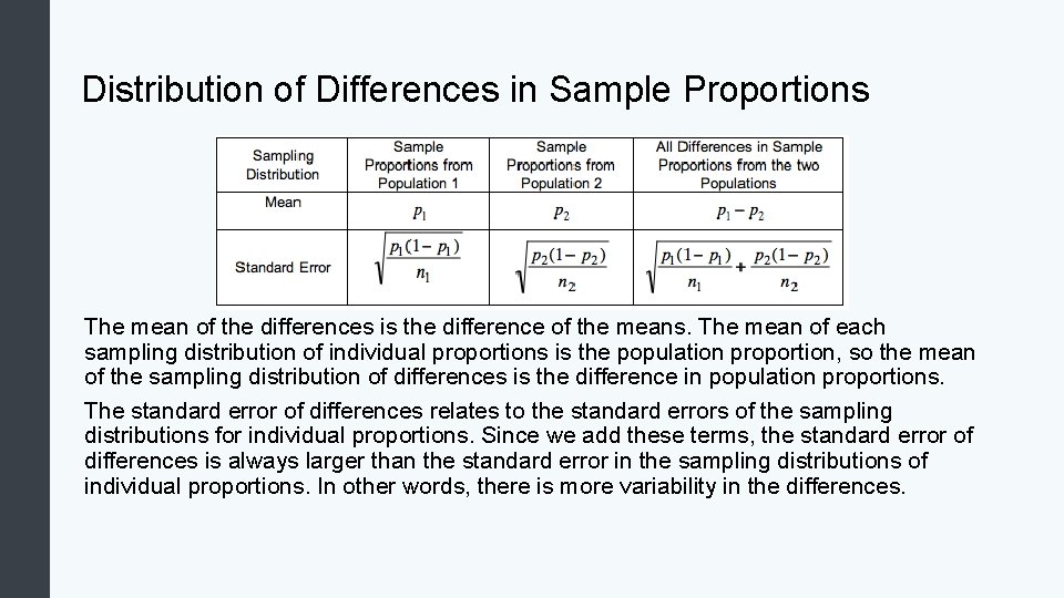
Distribution of Differences in Sample Proportions We want to create a mathematical model of the sampling distribution, so we need to understand when we can use a normal curve. We also need to understand how the center and spread of the sampling distribution relates to the population proportions. Shape: In each situation we have encountered so far, the distribution of differences between sample proportions appears somewhat normal, but that is not always true. We discuss conditions for use of a normal model later. Center: Regardless of shape, the mean of the distribution of sample differences is the difference between the population proportions, p 1 – p 2. This is always true if we look at the long-run behavior of the differences in sample proportions. Spread: We have observed that larger samples have less variability. Advanced theory gives us a formula for the standard error in the distribution of differences between sample proportions.

Distribution of Differences in Sample Proportions •

Distribution of Differences in Sample Proportions The mean of the differences is the difference of the means. The mean of each sampling distribution of individual proportions is the population proportion, so the mean of the sampling distribution of differences is the difference in population proportions. The standard error of differences relates to the standard errors of the sampling distributions for individual proportions. Since we add these terms, the standard error of differences is always larger than the standard error in the sampling distributions of individual proportions. In other words, there is more variability in the differences.

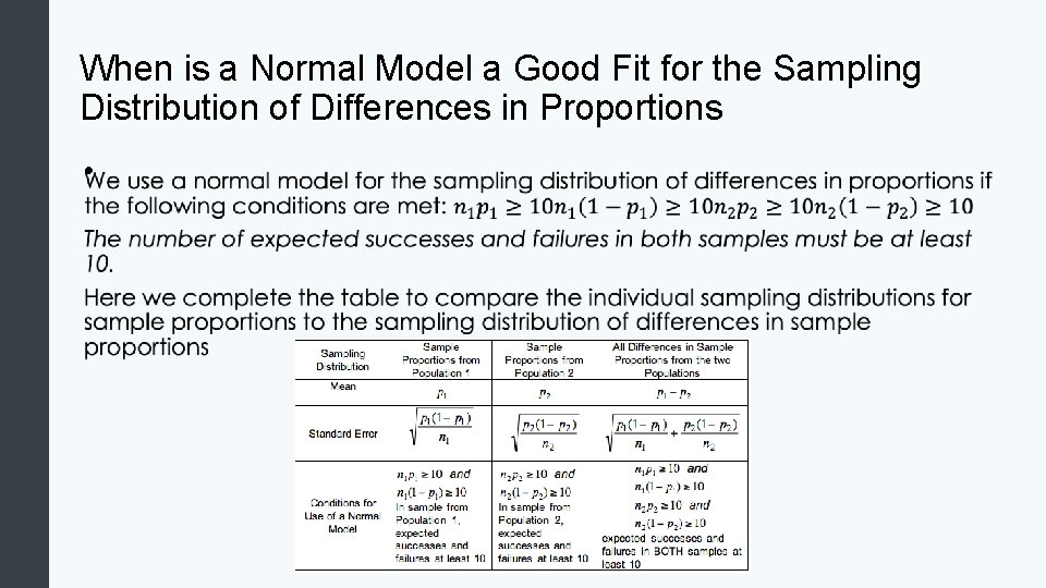
When is a Normal Model a Good Fit for the Sampling Distribution of Differences in Proportions •

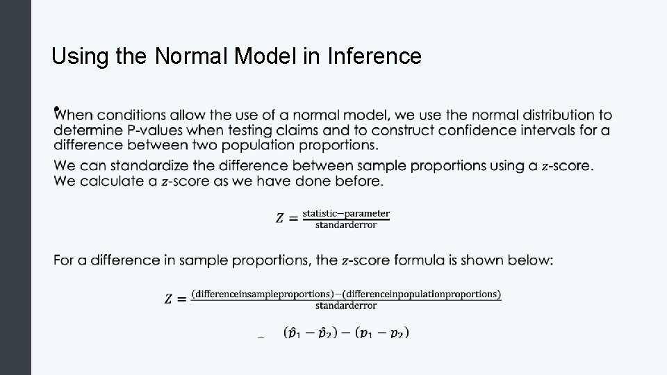
Using the Normal Model in Inference •

Confidence Interval for a Difference in Two Population Proportions: the Basics Every confidence interval has this form: statistic ± margin of error To estimate a difference in population proportions (or a treatment effect), the statistic is a difference in sample proportions, so the confidence interval is (difference in sample proportions) ± margin of error If a normal model is a good fit for the sampling distribution, we use the normal model to describe our confidence that the difference in population proportions lies within a given margin of error of the difference in sample proportions. For example, we can state that we are 95% confident that the difference in population proportions is contained in the following interval: (difference in sample proportions) ± 2(standard error)

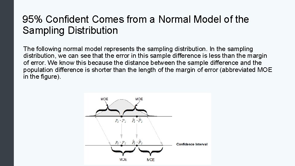
95% Confident Comes from a Normal Model of the Sampling Distribution The following normal model represents the sampling distribution. In the sampling distribution, we can see that the error in this sample difference is less than the margin of error. We know this because the distance between the sample difference and the population difference is shorter than the length of the margin of error (abbreviated MOE in the figure).

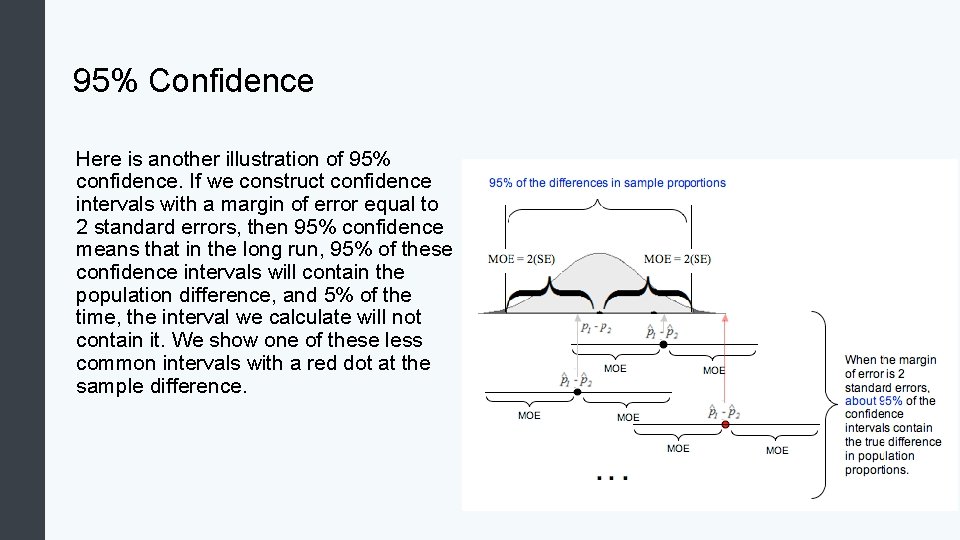
95% Confidence Here is another illustration of 95% confidence. If we construct confidence intervals with a margin of error equal to 2 standard errors, then 95% confidence means that in the long run, 95% of these confidence intervals will contain the population difference, and 5% of the time, the interval we calculate will not contain it. We show one of these less common intervals with a red dot at the sample difference.

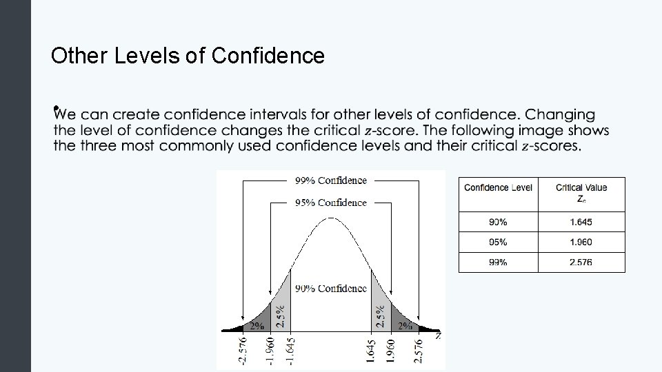
Other Levels of Confidence •

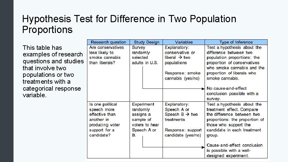
Hypothesis Test for Difference in Two Population Proportions This table has examples of research questions and studies that involve two populations or two treatments with a categorical response variable.

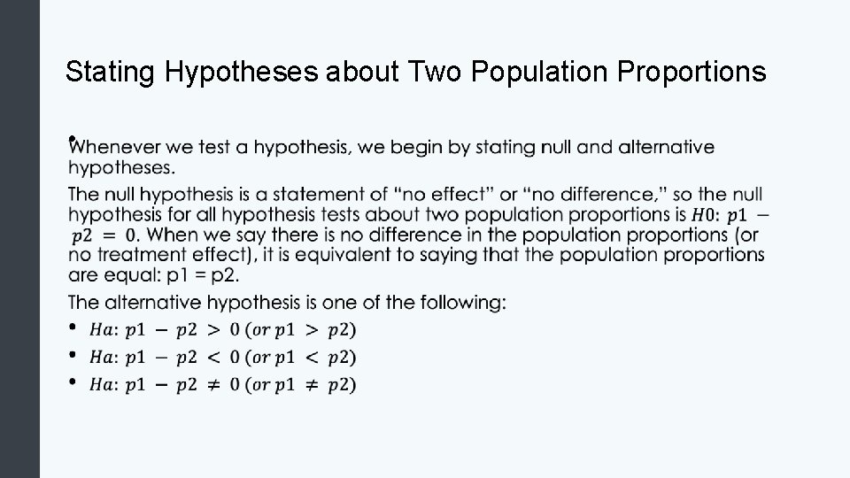
Stating Hypotheses about Two Population Proportions •

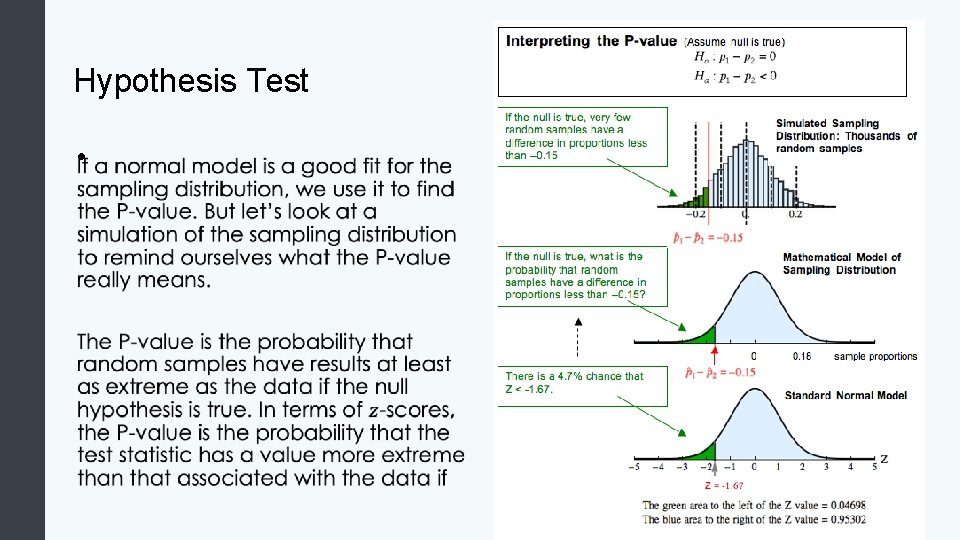
Hypothesis Test •

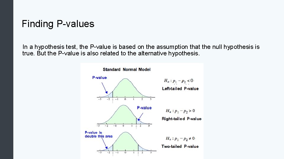
Finding P-values In a hypothesis test, the P-value is based on the assumption that the null hypothesis is true. But the P-value is also related to the alternative hypothesis.

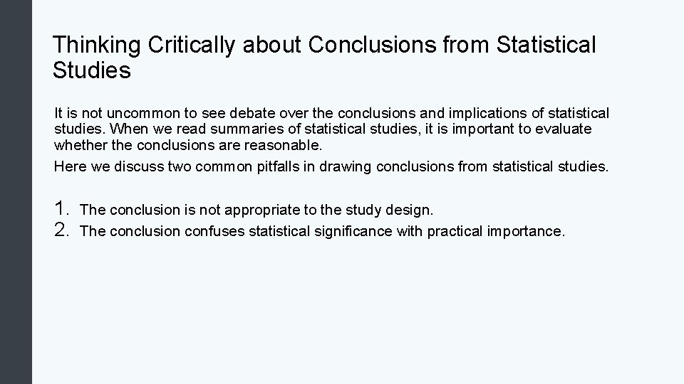
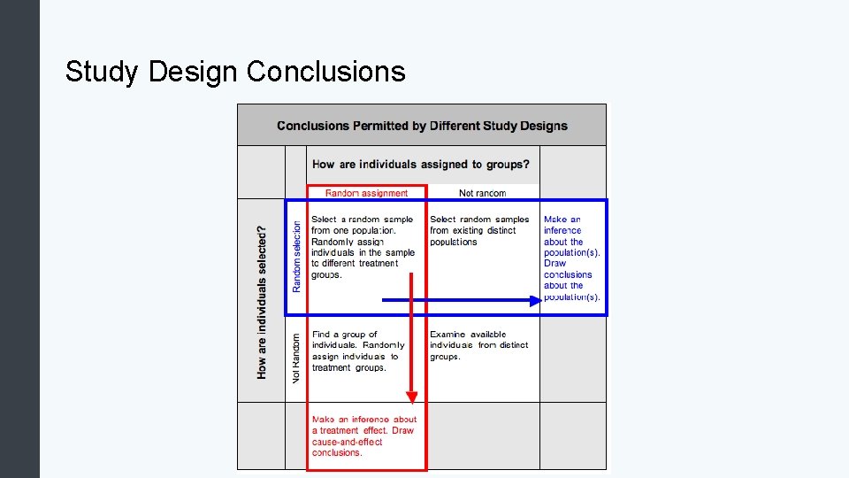
Thinking Critically about Conclusions from Statistical Studies It is not uncommon to see debate over the conclusions and implications of statistical studies. When we read summaries of statistical studies, it is important to evaluate whether the conclusions are reasonable. Here we discuss two common pitfalls in drawing conclusions from statistical studies. 1. 2. The conclusion is not appropriate to the study design. The conclusion confuses statistical significance with practical importance.

Study Design Conclusions

Statistical Significance and Practical Importance Is a statistically significant difference always large enough to be important on a practical level? The answer is no. Recall that when a P-value is less than the level of significance, we say the results are statistically significant. It means that the results are not due to chance. In the case of a difference in sample proportions, we are saying that the observed difference is larger than we expect to see in random samples from populations with the same population proportions. But this does not necessarily mean the difference is large enough to be important in real life.

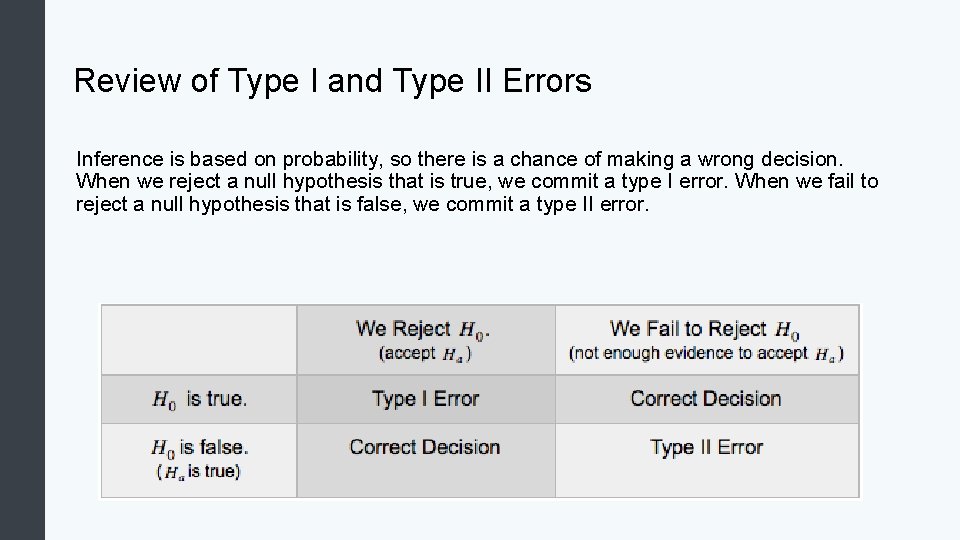
Review of Type I and Type II Errors Inference is based on probability, so there is a chance of making a wrong decision. When we reject a null hypothesis that is true, we commit a type I error. When we fail to reject a null hypothesis that is false, we commit a type II error.

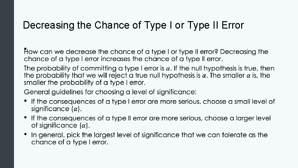
Decreasing the Chance of Type I or Type II Error •

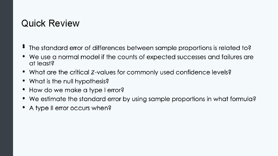
Quick Review •