Inference for Two Independent Sample Means Inference for

Inference for Two Independent Sample Means Inference for Two Samples 1

Introduction to Statistical Inference Methods � � Statistical Inference: Drawing conclusions about a population from sample data. Methods Ø Point Estimation– Using a sample statistic to estimate a parameter Ø Confidence Intervals – supplements an estimate of a parameter with an indication of its variability Ø Hypothesis Tests - assesses evidence for a claim about a parameter by comparing it with observed data Parameter Measure Statistic Mean of a single population Proportion of a single population Mean difference of two dependent populations (MP) Difference in means of two independent populations Difference in proportions of two populations Variance of a single population Standard deviation of a single population S

Independent Samples � Two samples are independent when the method of sample selection is such that those individuals selected for sample 1 do not have any relationship to those individuals selected for sample 2. � The samples are unrelated, uncorrelated. 3

Independent Samples assumptions: � With one sample tests, we compare a single sample mean to a known population mean (a value we believe to be true in the null hypothesis). � Now both population means, m 1 & m 2 are unknown. � We may be interested in the difference in treatments on the two groups as a whole. � Our parameter of interest would now be m 1 -m 2

Sampling Distribution of the difference in means � Suppose we had two normally distributed populations: � Heights of males in the US: � Heights of females in the US: ◦ X 1 ~ N(69, 3. 2) ◦ X 2 ~ N(64, 2. 8) �I built two sampling distributions (n=10) in Minitab. 5

6

Difference Distribution � 7

Difference Distribution This histogram represents the distribution of male mean heights subtracted from the distribution of female heights. 8

Sampling distribution of the difference in means: Large Samples � 9

Looking at differences in means Ways to analyze the mean difference � Create a comparative boxplot. � Run a formal 2 sample HT for µ 1= µ 2 to see if there is a difference. � If you find a difference, calculate a CI to estimate it 10

Hypothesis Test of the difference in means: Test Statistic �

Sampling distribution of the difference in means: Small Samples � 12

Hypothesis Test of the difference in means: Test Statistic �

� The Hypothesis Test of the difference in means: Hypotheses Null is the “No change” Hypothesis ◦ H 0: m 1 - m 2 =0 OR (m 1 = m 2) � Alternative options: ◦ Two Tailed test �Ha: m 1 – m 2 ≠ 0 or (m 1 ≠ m 2) ◦ One Tailed test �Ha: m 1 – m 2 > 0 or (m 1 > m 2 ) �Ha: m 1 – m 2 < 0 or (m 1 < m 2 )

Degrees of Freedom? � Easiest to just use a “conservative estimate”: Min{n 1– 1, n 2– 1} � There is also more precise way of calculating 2 independent sample df, although you will most likely not want to deal with this by hand:

Two sample means hypothesis test � Suppose that a school district is interested in comparing standardized test scores for two high schools (East and West) having different curriculums. A sample of students is taken from both schools. The data is summarized as follows: n Mean S East HS 24 84 8. 78 West HS 26 78. 34 7. 553

Stating Hypotheses � It is unclear which school will achieve high scores. � The null states that the population means for the two groups are equal. � Consider a two-tailed hypothesis test H 0: m 1 – m 2 = 0 or m 1 = m 2 Ha: m 1 – m 2 ≠ 0 or m 1 ≠ m 2 � As � usual, we will state a = 0. 05. It does not matter which group we designate as group 1 or 2.

Check Conditions � Check your assumptions for t visually � Graph each sample to check conditions:

Test Statistic n Mean S East HS 24 84 8. 78 West HS 26 78. 34 7. 553

Critical Value � We need a T Critical value with: ◦ df=min {n 1 -1, n 2 -1) = min{24 -1, 26 -1} = 23 ◦ a = 0. 05 ◦ Two-Tailed � Table Value ◦ ± 2. 069 21

P-value � We need 2*P(t > 2. 437) � Estimating w/ table ◦ df=min {n 1 -1, n 2 -1)= min{24 -1, 26 -1} = 23 ◦ 2*(0. 01)<-p-val< 2*(0. 025) => 0. 02<-p-val< 0. 05 � By Technology: ◦ 0. 02296

Conclusion � Test � The Statistic is in Rejection Region p-value is 0. 023 < 0. 05, reject the null hypothesis � The difference between the two groups is “statistically significant. ” � This means there is a difference in the two curriculum 23

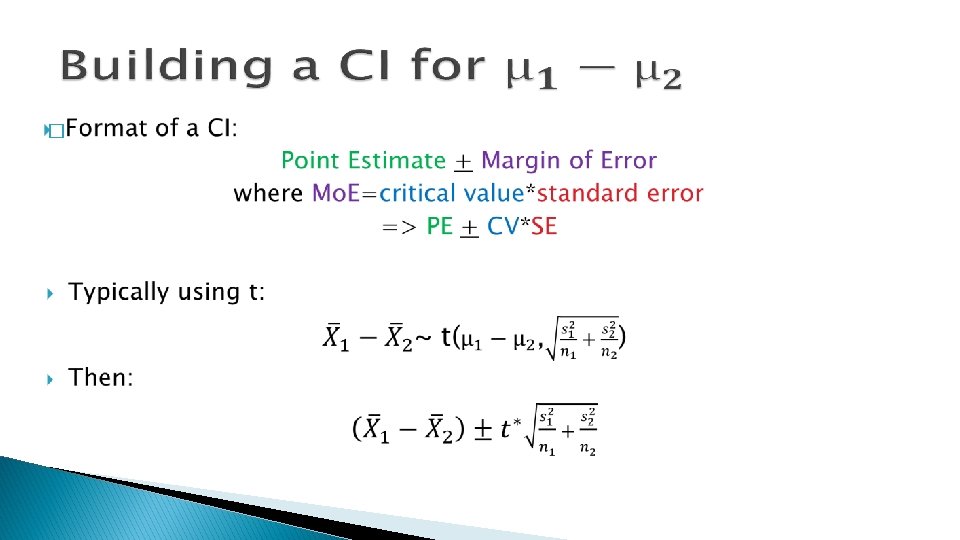
Estimating the difference: CI for m 1 - m 2 � Now that we have found a difference, let’s estimate it. � Construct a 95% CI for the difference in means � Recall n Mean S East HS 24 84 8. 78 West HS 26 78. 34 7. 553 df=min {n 1 -1, n 2 -1)= min{24 -1, 26 -2} = 23 the sample statistics: � Plugging in: � Interpret: ◦ We are 95% confident the true difference in means is captured by this interval 24