Inference for contigency tables Chapter 3 LOGO introduction

Inference for contigency tables Chapter 3 LOGO

introduction In this chapter we introduce inferential methods for contingency tables. The methods assume Poisson, multinomial, or independent binomial sampling.

3. 1 CONFIDENCE INTERVALS FOR ASSOCIATION PARAMETERS The accuracy of estimators of association parameters is characterized by standard errors of their sampling distributions. In this section we present large-sample standard errors and confidence intervals, focusing on paramters for 2× 2 tables.

Interval Estimation of Odds Ratios sample odds ratio for a 2× 2 tables: Its distribution is very skewed unless n is large.

Interval Estimation of Odds Ratios log transform: 1. having an additive rather than multiplicative structure 2. Converges more rapidly to normality. estimated standard error: Wald confidence interval:

If an nij= 0 : 1. =0 or undefined. 2. Wald interval does not exist but by some adjustment …. 3. Confidence intervals formed by inverting the score test or likelihood ratio test it is not problematic. In this case…. .

Example: seat-belt use The estimate is imprecise because ….

Interval Estimation of Difference of Proportions and relative risk The difference of proportions and the relative risk compare conditional distributions of a response variable for two groups. In this case we treat the samples as independent binomials. For group i : yi has a binomial distribution with sample size ni and a probability Πi.

Interval Estimation of Difference of Proportions it usually has true coverage probability less than the nominal confidence coefficient, especially when Π 1 , Π 2 are near 0 or 1.

Interval Estimation of Relative Risk sample relative risk: ü Like the odds ratio, it converges to normality faster on the log scale. asymptotic standard error of log r : Wald interval for log r: ü It is somewhat conservative.

example v According to either measure benefits could result from taking aspirin. v The estimate is imprecise because ….

Deriving Standard Errors with the Delta Method It is a a simple method for deriving standard errors for large-sample inferences. Tn ~ N ( θ , ) (asymptoticaly) Suppose : estimator is a function g(Tn ) of Tn. Then g(Tn ) has a large-sample normal distribution. The standard error depends on how fast g(t) changes for t near θ. for large n, suppose that Tn ~ N ( θ , ) then :

Deriving Standard Errors with the Delta Method Let g be a function that is at least twice differentiable at θ. Using the Taylor series in a neighborhood of t = θ , Recall 1 : Recall 2 : Thus : g(Tn ) ~ N ( g(θ) , )

Deriving Standard Errors with the Delta Method

Delta Method Applied to Sample Logit delta method for a function of the ML estimator Tn = parameter for y successes in n trials. = y / n of the binomial has a large-sample normal distribution by the central limit theorem. So do many functions of.

Delta Method for Log Odds Ratio Standard errors for the log odds ratio and the log relative risk result from a multiparameter version of the delta method. Suppose : sample proportion : have a large-sample multivariate normal distribution. Since odds ratio is a function of them, the delta method implies in this way :

Delta Method for Log Odds Ratio Let denote a differentiable function of multinomial sample. Let with sample value for a

Delta Method for Log Odds Ratio applying the delta method to the log odds ratio :

Simultaneous confidence intervals for multiple comparison Multiple comparison methods apply the confidence level to the simultaneous set of all comparison, rather than to each individual one.

TESTING INDEPENDENCE IN TWO-WAY CONTINGENCY TABLES We assume multinominal sampling with joint probabilitis in an I × J contigency table. The null hypothesis of statistical independence is : For all i , j

Pearson and likelihood–ratio chi-squared test X statistics was introduced to test specified values of multinominal probabilities. Here we apply it to test H 0 : independence X 2 is asymptotically chi-squared with df= IJ -1 but …
(J-1)")
Pearson and likelihood–ratio chi-squared test Likelihood ratio test : df=(I-1)(J-1)

Pearson and likelihood–ratio chi-squared test X 2 and G 2 they are then asymptotically equivalent; X 2 - G 2 converges in probability to zero. When there are independent multinomial samples in rows …. . When there are independent multinomial samples in columns …. . When the condition is on both row and column marginal total …. .

example

www. Win 2 Farsi. com Adequacy of chi-squared tests q As n grows , the multinomial distribution for {nij} is better approximated by a multivariate normal, and X 2 and G 2 have more nearly chi-squared distributions for fixed number of cells. q The adequacy of the approximation depends on …. . q Sparse contigency tables : … q With small n and more sparse table X 2 performs better than G 2. q The approximation is usually poor for G 2 when ( n / IJ ) < 5. q A caveat is that chi-squared approximations tend to be poor for tables containing both very small and moderately large. q Small-sample methods are available whenever it is doubtful whether n is sufficiently large. Company name

Adequacy of chi-squared tests

chi-squared and comparing proportions in 2× 2 tables summarizes results for 2 binomial variates , y 1 and y 2 with n 1 and n 2 trials. H 0 : Independent = homogenity ( ) Under H 0 the estimated common value for Z score statistics: In 2× 2 tables Z 2 = X 2. A formula for X 2 in 2× 2 tables: is : ~ N

www. Win 2 Farsi. com Score confidence intervals comparing prportions Wald confidence intervals are simple but have some disadvantages : i. They are dependent on the scale of measurment. For example …. ii. They fail when an estimate falls at the boundary of parameter space. For example …. iii. Sometimes the actual probability of covering the parameter is far from the nominal level unless n is large. intervals result from score test or likelihood ratio test do not have these disadvantages. Company name

Score and confidence intervals comparing prportions score method for the difference of proportions :

Score and confidence intervals comparing prportions score method for odds ratio in 2× 2 tables :

Profile Likelihood Confidence Intervals

Profile Likelihood Confidence Intervals

FOLLOWING-UP CHI-SQUARED TESTS chi-squared tests of independence have limited usefulness: A small P-value indicates …. So don’t rely solely on results of chi-squared tests rather than studying the nature of the association.

Pearson and Standardized Residuals A cell-by-cell comparison of observed and estimated expected frequencies helps show the nature of the dependence. The Pearson residual, defined for a cell by A standardized Pearson residual that is asymptotically standard normal results from dividing it by its standard error. For H 0: independence, this is > 2 or 3

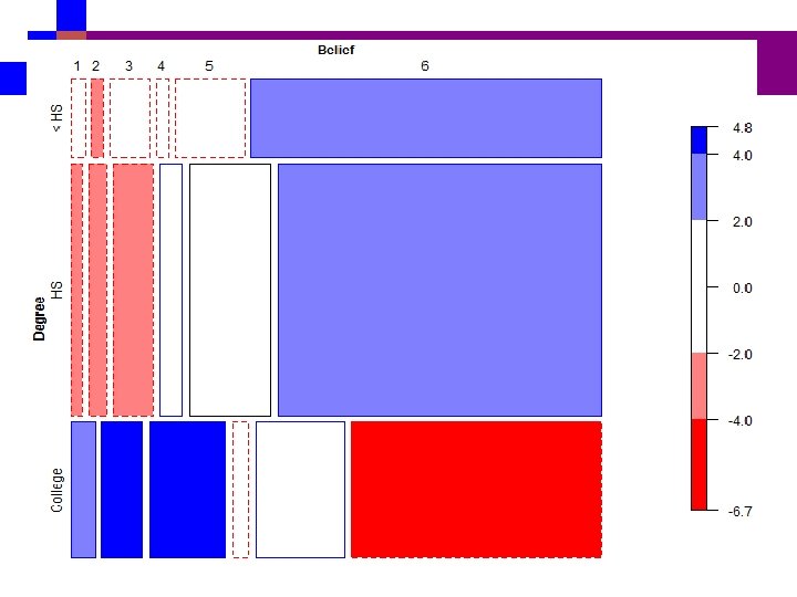
Education and blief in God Revisited

www. Win 2 Farsi. com Education and blief in God Revisited Company name

Partitioning Chi-Squared Use reproductivity propertyto partition G 2. ü partitioning G 2 (with df= J-1) in 2×J tables : computing G 2 for J-1 2× 2 tables.

Partitioning Chi-Squared In I×J tables : 1. independent chi-squared components result from comparing columns 1 and 2 and …. Then we have (J-1) statistics with df= I-1. 2. More refined method produce (J-1)(I-1) 2× 2 tables.

Origin of Schizophrenia Example Here G 2=23. 04 with df=4. To understand this association better, we partition G 2 into four independent components G 2= 0. 29 G 2= 1. 36 G 2= 12. 95 G 2= 8. 43 23. 04

Rules for Partitioning For forming subtables determining independent components of chi-squared : 1. The df for the subtables must sum to df for the full table. 2. Each cell count in the full table must be a cell count in one and only one subtable. 3. Each marginal total of the full table must be a marginal total for one and only one subtable.

Some points q when the subtable df values sum properly but the G 2 values do not, the components are not independent. q For the G 2 statistic, exact partitionings occur. q The Pearson X 2 need not equal the sum of the X 2 values for the subtables. q When the null hypotheses all hold, X 2 does have an asymptotic equivalence with G 2. q when the table has small counts in large-sample chi-squared tests it is safer to use X 2 to study the subtables.

Summarizing the association

Limitations of Chi-Squared Tests v Chi-squared tests of independence merely indicate the degree of evidence of association. They are rarely adequate for answering all questions about a data set. v To investigate the nature of the association: Study residuals, decompose chisquared into components, and estimate parameters such as odds ratios that describe the strength of association. v chi-squared tests require large samples. v chi-squared tests both classifications as nominal because used in X 2 and G 2 depend on the marginal totals but not on the order of listing the rows and columns. X 2 and G 2 do not change value with arbitrary reorderings of rows or of columns

Why Consider Independence? Ø Any idealized structure such as independence is unlikely to hold in any given practical situation. Ø One reason refers to the benefits of model parsimony. Fewer parameter used to describe the data. Ø The independence ML estimates smooth the sample counts, somewhat damping the random sampling fluctuations. Independence estimators can have smaller MSE according to :

TWO-WAY TABLES WITH ORDERED CLASSIFICATIONS The X 2 and G 2 chi-squared tests ignore some information when used to test independence between ordinal classifications. When rows and/or columns are ordered, more powerful tests usually exist.

Linear Trend Alternative to Independence When the row variable X and the column variable Y are ordinal, a positive or negative trend in the association is common. Detecting a linear trend alternative to independence requires assigning scores to X and Y, treating them as interval variables. scores for the rows: scores for the column: scores have the same ordering as the categories This statistic utilizes correlation information in a way that : correlation r between X and Y equals the standardization of this sum to the -1 to +1 scale.

Linear Trend Alternative to Independence H 0 : r=0 H 1 : r ≠ 0 For large samples, it is approximately chi-squared with df=1. Large values contradict independence. A small P-value does not imply that the association is linear, merely that the linear component of the association is significant.

Example: Is happiness associated with political ideology? X 2= 7. 07 P-values= 0. 13 statistics show little evidence of association, but they ignore the ordering of rows and columns Scores : {1, 2, 3} r= 0. 135 P= 0. 016

Monotone Trend Alternatives to Independence To survey Monotone Trend : uses an ordinal measure of association, such as gamma. For large random samples, sample gamma has approximately a normal sampling distribution. The standard error SE follows from the delta method A confidence interval describes the strength of positive or negative monotone association. Back to the example:

Extra Power with Ordinal Tests For testing independence, X 2 and G 2 refer to the most general alternative. in X 2 and G 2 : df = (I-1)(J-1). In achieving this generality, they sacrifice sensitivity for detecting particular patterns. the analyses for ordinal row and column variables use a single parameter. For instance, M 2 uses the correlation (it has df=1). When the association truly has a positive or negative trend, an ordinal test has a power advantage over the tests using X 2 or G 2. because : a relatively large M 2 value with df=1 falls farther out in its right-hand tail than a comparable value of X 2 or G 2 with df=(I-1)(J-1) , produces a smaller P-value. The potential discrepancy in power increases as I and J increase.

Sensitivity to choice of scores Often, it is unclear how to assign scores to statistics that require them, such as M 2. Cochran. noted that ‘‘any set of scores gives a valid test, provided that they are constructed without consulting the results of the experiment. If the set of scores is poor the test will not be sensitive. the scale is chosen by a consensus of experts

Sensitivity to choice of scores How sensitive are analyses to the choice of scores? q There is no simple answer, but different choice of monotone scores can give similar results. q Scores that are linear transforms of each other, such as (1, 2, 3, 4) and (0, 2, 4, 6) , have the same absolute correlation and hence the same M 2. q Results may depend on the scores, however, when the data are highly unbalanced, with some categories having many more observations than others.

Example: infant birth defects by maternal alcohol consumption When a variable is nominal but has only two categories, statistics (such as M 2) that treat the variable as ordinal are still valid (malforation). alcohol consumption is ordinal (continuous var)

www. Win 2 Farsi. com Example: infant birth defects by maternal alcohol consumption Company name

www. Win 2 Farsi. com Example: infant birth defects by maternal alcohol consumption Company name

Trend Tests for I× 2 and 2×J Tables When I or J equal 2, the tests based on linear or monotonic trend simplify. With binary X, 2×J tables occur in comparisons of two groups, such as when the rows represent two treatments Using scores {u 1=0, u 2=1} for levels of X, the covariation measure in M 2 simplifies to proportion of subjects in row 2 mean score for that row M 2 : detecting differences between the two row means of the scores on Y. Wilcoxon or Mann. Whitney test

Trend Tests for I× 2 and 2×J Tables This test is also asymptotically equivalent to test statistics based on the numbers of concordant and discordant pairs. z=(C-D)/SE 0 The square of the statistic is equivalent to M 2. Related measures such as difference between 2 groups. is also relevant to detect the When Y has two levels, the table has size I× 2. The linear trend statistic then refers to a linear trend in the probability of either response category.

Nominal–Ordinal Tables The tests using the correlation or gamma are appropriate when both classifications are ordinal. When one is nominal with more than two categories, other statistics are needed.

SMALL-SAMPLE TESTS OF INDEPENDENCE The inferential methods of the preceding four sections are large-sample methods. When n is small, alternative methods use exact small-sample distributions rather than large-sample approximations.

Fisher’s Exact Test for 2× 2 Tables This test is a small-sample tests of independence. To test the independence, conditioning on both sets of marginal totals in a table that yields the hypergeometric distribution t 0 n 1+ n 2+ n+1 n+2 For 2× 2 tables, independence is equivalent to the odds ratio θ=1. H 0 : θ=1 H 1 : θ>1 Tables having larger n 11 have larger sample odds ratios and hence stronger evidence in favor of Ha. If n 11 = t 0 , P-value : p ( n 11 ≥ t 0 )

Example: Fisher’s Tea Drinker Claim : when drinking tea she could distinguish whether milk or tea was added to the cup first. To test her claim …. The experimental design fixed both marginal distributions, since …. H 0 : θ=1 H 1 : θ>1 Thus, the hypergeometric applies naturally for the null distribution of n 11. The P-value is :

Two-Sided P-Values for Fisher’s Exact Test For a two-sided P-value : 1. a popular approach sums P(n 11 = t ) for counts t such that p(t ≤ to ) ; that is, the P-value is : 2. 3. 4. plus an attainable probability in the other tail that is as close as possible to, but not greater than, that one-tailed probability.

Two-Sided P-Values for Fisher’s Exact Test Each approach has advantages and disadvantages. They can provide different results because of the discreteness and potential skewness. In practice, two-sided tests are much more common than one-sided. To conduct a test of size 0. 05 when one truly believes that the effect has a particular direction, it is safest to conduct the one-sided test at the 0. 025 level.

Confidence intervals based on conditional likelihood :

Discreteness and Conservatism Issues The hypergeometric distribution is highly discrete for small samples, as n 11 and hence the P-value can assume relatively few values. It is usually not possible to achieve a fixed significance level such as 0. 05. In the tea-tasting experiment : n 11 can equal only 4, 3, 2, 1, 0 one-sided P-values are restricted to : 0. 014, 0. 243, 0. 757, 0. 986, and 1. 0 Only the P-value of 0. 014 does not exceed 0. 05; thus, when H 0 is true, the probability of falsely rejecting it is 0. 014, not 0. 05. In this sense, the traditional approach to hypothesis testing is conservative: The true probability of type I error is less than the nominal level.

Discreteness and Conservatism Issues It is possible to achieve any fixed significance level by data-unrelated randomization on the boundary of the critical region, in deciding whether to reject H 0. For the tea-tasting experiment: suppose that we reject H 0 when n 11 =4, we reject H 0 with probability 0. 157 when n 11= 3, and we do not reject H 0 otherwise. when n 11 = 3, we generate a uniform random variable U over [0, 1] and reject H 0 if U < 0. 157 1 ˠ 0 x>3 x=3 o. w

Discreteness and Conservatism Issues With the randomization extension, it is showed that Fisher’s test is uniformly most powerful unbiased We recommend simply reporting the P-value. To reduce conservativeness, report the mid-P-value. For the one-sided test with the tea-tasting data The test is no longer guaranteed to have true (type I error) no greater than the nominal value, but in practice it is rarely much greater.

Small-Sample Unconditional Test of Independence A common sampling assumption for analyses comparing two groups on a binary response is that the rows are independent binomial samples. Then, Only { ni+ } are naturally fixed. An alternative small-sample test, designed for independent binomial samples, conditions on only the row totals. Under binomial sampling with parameter in row i, consider testing: using some test statistic T, such as the Pearson X 2 and

Small-Sample Unconditional Test of Independence We illustrate using test statistic X 2 for the 2× 2 table : This X 2 value for the observed table and for table The probability of the first table is: The probability of the second table is: 0 3 3 0 0 3 X 2 =6 is the maximum possible.

Conditional versus Unconditional Test

www. Win 2 Farsi. com Conditional versus Unconditional Test Company name

Beysian inference for two-way contigency tables

Prior distribution for comparing proportions in 2× 2 tables.

Prior distribution for comparing proportions in 2× 2 tables.

Posterior probabilities comparing proportions

Posterior probabilities comparing proportions

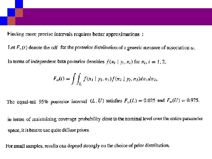
Posterior intervals for association parameter

example 11 0 0 1

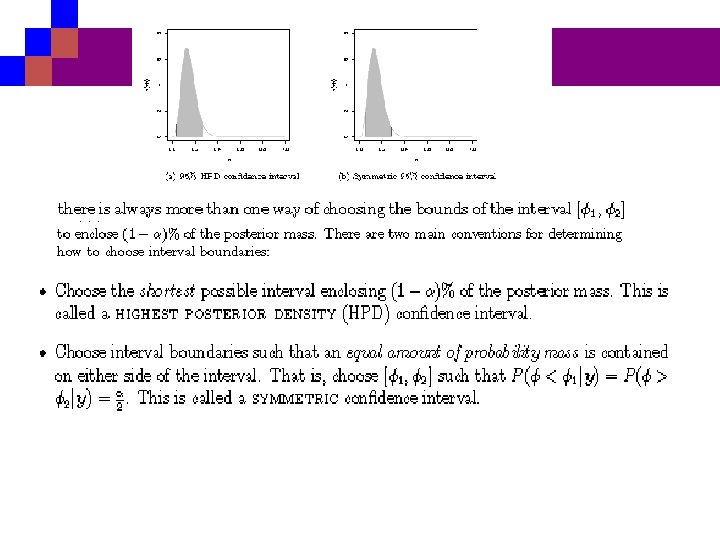
Highest posterior density intervals

Testing independence

Empirical bayes and hierarchical beysian approaches

Extentions for multiway tables and nontabulated response.

Categorical data need not be contigency tables.

ﺭﺳﻢ ﻧﻤﻮﺩﺍﺭ ﻣﻮﺯﺍﺋیکی x<- c(9, 8, 27, 8, 47, 236, 23, 39, 88, 49, 179, 706, 28, 48, 89, 104, 293) data <- matrix(x, nrow=3, ncol=6, byrow=TRUE) dimnames(data) = list(Degree=c("< HS", "College"), Belief=c("1", "2", "3", "4", "5", "6")) install. packages("vcd. Extra") library("vcd. Extra") ﻣﺎﻧﺪﻩﻫﺎی ﺍﺳﺘﺎﻧﺪﺍﺭﺩﺷﺪﻩ Std. Resid <- c(-0. 4, -2. 2, -1. 4, -1. 5, -1. 3, 3. 6, -2. 5, -2. 6, 3. 3, 1. 8, 0. 0, 3. 4, 3. 1, 4. 7, 4. 8, -0. 8, 1. 1, -6. 7) Std. Resid <- matrix(Std. Resid, nrow=3, ncol=6, byrow=TRUE) mosaic(data, residuals = Std. Resid, gp=shading_Friendly) mosaic

ﺍﻃﻼﻋﺎﺗی ﺩﺭ ﻣﻮﺭﺩ ﺗﻮﺯیﻊ پیﺸیﻦ v Noninformative Priors Prio A prior distribution is noninformative if the prior is "flat" relative to the likelihood function(if it has minimal impact on the posterior distribution). Other names for the noninformative prior are vague, diffuse, and flat prior. v Improper Priors A prior is said to be improper if For example, a uniform prior distribution on the real line is an improper prior.

v Conjugate Priors A prior is said to be a conjugate prior for a family of distributions if the prior and posterior distributions are from the same family, which means that the form of the posterior has the same distributional form as the prior distribution. v Informative priors An informative prior is a prior that is not dominated by the likelihood and that has an impact on the posterior distribution.

The Bayes factor v The Bayes Factor provides a way to formally compare two competing models, say M 1 and M 2. v Given a data set x, we compare models v We may specify prior distributions p 1(1) and p 2(2) that lead to prior probabilities for each model p(M 1) and p(M 2).

The Bayes factor The Bayes Factor is: (the ratio of the posterior odds for M 1 to the prior odds for M 1).


- Slides: 93