INF 1060 SPREADSHEET 1 INF 1060 SPREADSHEET 1

INF 1060: SPREADSHEET 1

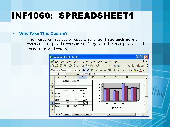
INF 1060: SPREADSHEET 1 • Why Take This Course? – This course will give you an opportunity to use basic functions and commands in spreadsheet software for general data manipulation and personal record keeping.

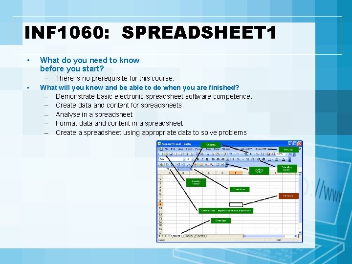
INF 1060: SPREADSHEET 1 • • What do you need to know before you start? – There is no prerequisite for this course. What will you know and be able to do when you are finished? – Demonstrate basic electronic spreadsheet software competence. – Create data and content for spreadsheets. – Analyse in a spreadsheet – Format data and content in a spreadsheet – Create a spreadsheet using appropriate data to solve problems

INF 1060: SPREADSHEET 1 • When should your work be done? – This module should take approximately 20 hours to complete.

INF 1060: SPREADSHEET 1 • Which resources can you use? – Microsoft Excel 2010 – Assignment templates found in the Information Processing 10 folder – The help menu, …. . – This on-line tutorial http: //www. usd. edu/trio/tut/excel/index. html

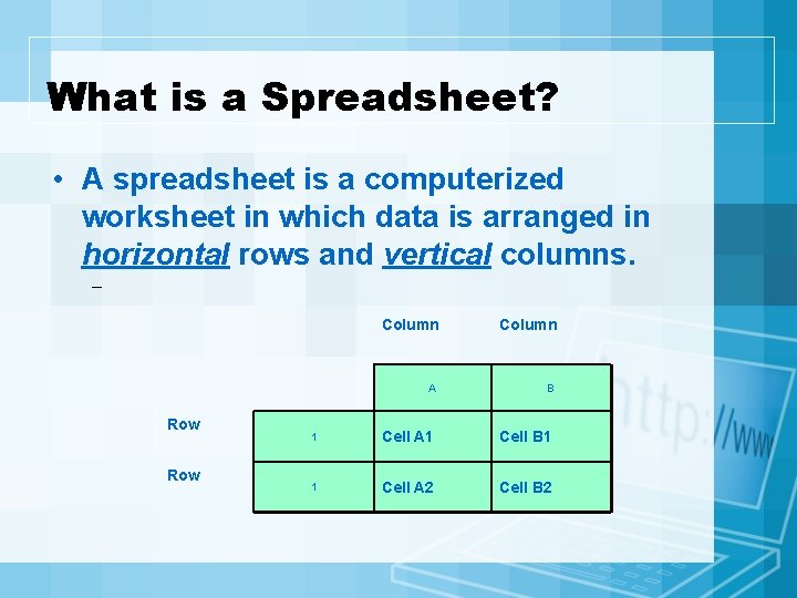
What is a Spreadsheet? • A spreadsheet is a computerized worksheet in which data is arranged in horizontal rows and vertical columns. – Row Column A B 1 Cell A 1 Cell B 1 1 Cell A 2 Cell B 2

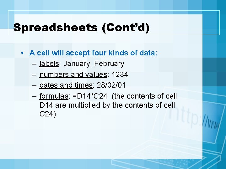
Spreadsheets (Cont’d) • A cell will accept four kinds of data: – labels: January, February – numbers and values: 1234 – dates and times: 28/02/01 – formulas: =D 14*C 24 (the contents of cell D 14 are multiplied by the contents of cell C 24)

Spreadsheets (Cont’d) • Spreadsheets automatically recalculate when data is changed via formulas. • Spreadsheets can be used for a variety of tasks. – For example, they can answer “what if” types of questions, such as the following: What happens if your allowance changed? • Once a spreadsheet has been created, it can be saved and used over and over. This is called a template.

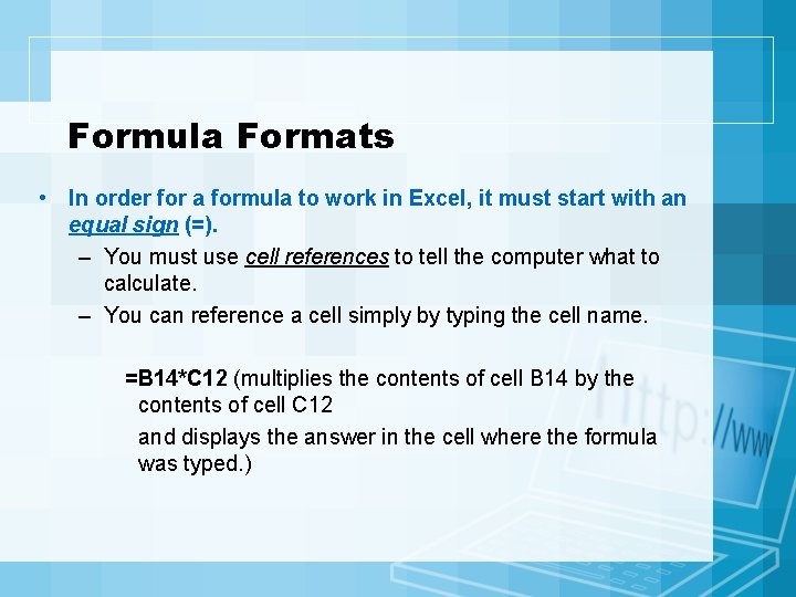
Formula Formats • In order for a formula to work in Excel, it must start with an equal sign (=). – You must use cell references to tell the computer what to calculate. – You can reference a cell simply by typing the cell name. =B 14*C 12 (multiplies the contents of cell B 14 by the contents of cell C 12 and displays the answer in the cell where the formula was typed. )

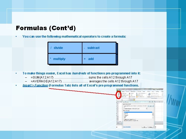
Formulas (Cont’d) • • • You can use the following mathematical operators to create a formula: / divide - subtract * multiply + add To make things easier, Excel has hundreds of functions pre-programmed into it: – =SUM(A 12: A 17) ………………sums the cells A 12 through A 17 – =AVERAGE(A 12: A 17) …………. averages the cells A 12 through A 17 Insert > Function (Formulas Tab) lists all of Excel’s pre-programmed functions.

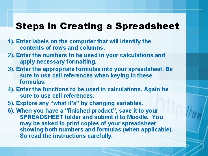
Steps in Creating a Spreadsheet 1). Enter labels on the computer that will identify the contents of rows and columns. 2). Enter the numbers to be used in your calculations and apply necessary formatting. 3). Enter the appropriate formulas into your spreadsheet. Be sure to use cell references when keying in these formulas. 4). Enter the functions to be used in calculations. Again be sure to use cell references. 5). Explore any “what if’s” by changing variables. 6). When you have a “finished product”, save it to your SPREADSHEET folder and submit it to Moodle. You may be asked to print copies of your spreadsheet showing both numbers and formulas (when applicable). So read the instructions carefully.

Formatting • • • Borders Merge and Center Change cell size Adding and Deleting Adding Sheets Saving

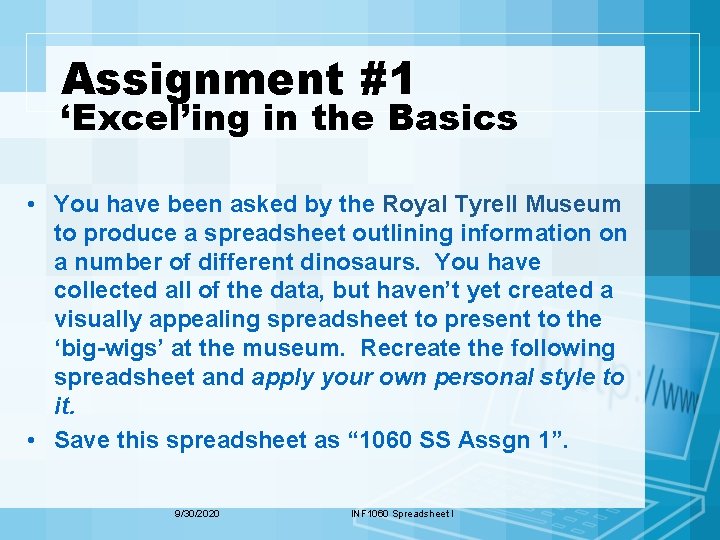
Assignment #1 ‘Excel’ing in the Basics • You have been asked by the Royal Tyrell Museum to produce a spreadsheet outlining information on a number of different dinosaurs. You have collected all of the data, but haven’t yet created a visually appealing spreadsheet to present to the ‘big-wigs’ at the museum. Recreate the following spreadsheet and apply your own personal style to it. • Save this spreadsheet as “ 1060 SS Assgn 1”. 9/30/2020 INF 1060 Spreadsheet I

9/30/2020 INF 1060 Spreadsheet I

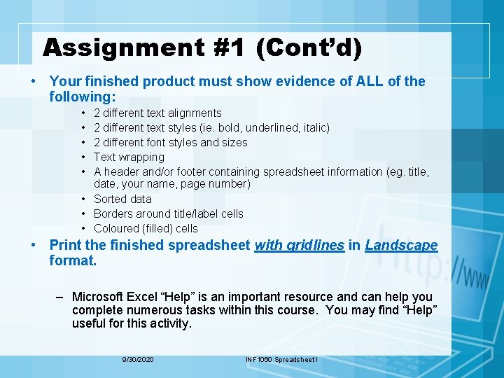
Assignment #1 (Cont’d) • Your finished product must show evidence of ALL of the following: • • • 2 different text alignments 2 different text styles (ie. bold, underlined, italic) 2 different font styles and sizes Text wrapping A header and/or footer containing spreadsheet information (eg. title, date, your name, page number) • Sorted data • Borders around title/label cells • Coloured (filled) cells • Print the finished spreadsheet with gridlines in Landscape format. – Microsoft Excel “Help” is an important resource and can help you complete numerous tasks within this course. You may find “Help” useful for this activity. 9/30/2020 INF 1060 Spreadsheet I

Assignment #2 The Fill Down Command • In this activity you will prepare a spreadsheet that calculates the net pay for each of the five employees of Crestwood Laundry for the week ending September 19, 2000. • Also, total the columns for Gross Pay, Income Tax, EI, Medical and Net Pay. 9/30/2020 INF 1060 Spreadsheet I

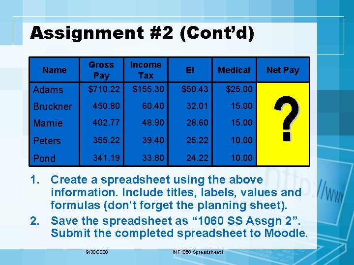
Assignment #2 (Cont’d) Gross Pay Income Tax $710. 22 $155. 30 $50. 43 $25. 00 Bruckner 450. 80 60. 40 32. 01 15. 00 Marnie 402. 77 48. 90 28. 60 15. 00 Peters 355. 22 39. 40 25. 22 10. 00 Pond 341. 19 33. 80 24. 22 10. 00 Name Adams EI Medical Net Pay 1. Create a spreadsheet using the above information. Include titles, labels, values and formulas (don’t forget the planning sheet). 2. Save the spreadsheet as “ 1060 SS Assgn 2”. Submit the completed spreadsheet to Moodle. 9/30/2020 INF 1060 Spreadsheet I

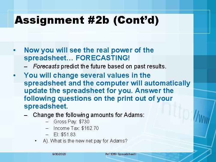
Assignment #2 b (Cont’d) • Now you will see the real power of the spreadsheet… FORECASTING! – Forecasts predict the future based on past results. • You will change several values in the spreadsheet and the computer will automatically update the spreadsheet for you. Answer the following questions on the print out of your spreadsheet. – Change the following amounts for Adams: • – Gross Pay: $730 – Income Tax: $162. 70 – EI: $51. 83 A). What is the new net pay for Adams? 9/30/2020 INF 1060 Spreadsheet I

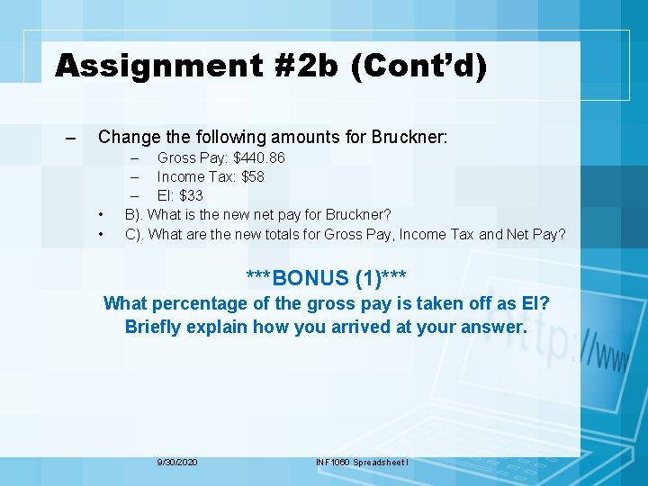
Assignment #2 b (Cont’d) – Change the following amounts for Bruckner: • • – Gross Pay: $440. 86 – Income Tax: $58 – EI: $33 B). What is the new net pay for Bruckner? C). What are the new totals for Gross Pay, Income Tax and Net Pay? ***BONUS (1)*** What percentage of the gross pay is taken off as EI? Briefly explain how you arrived at your answer. 9/30/2020 INF 1060 Spreadsheet I

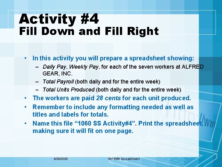
Activity #4 Fill Down and Fill Right • In this activity you will prepare a spreadsheet showing: – Daily Pay, Weekly Pay, for each of the seven workers at ALFRED GEAR, INC. – Total Payroll (both daily and for the entire week) – Total Units Produced (both daily and for the entire week) • The workers are paid 28 cents for each unit produced. • Remember to include any formatting needed as well as titles and labels for totals. • Name this file “ 1060 SS Activity#4”. Print the spreadsheet, making sure it will fit on one page. 9/30/2020 INF 1060 Spreadsheet I

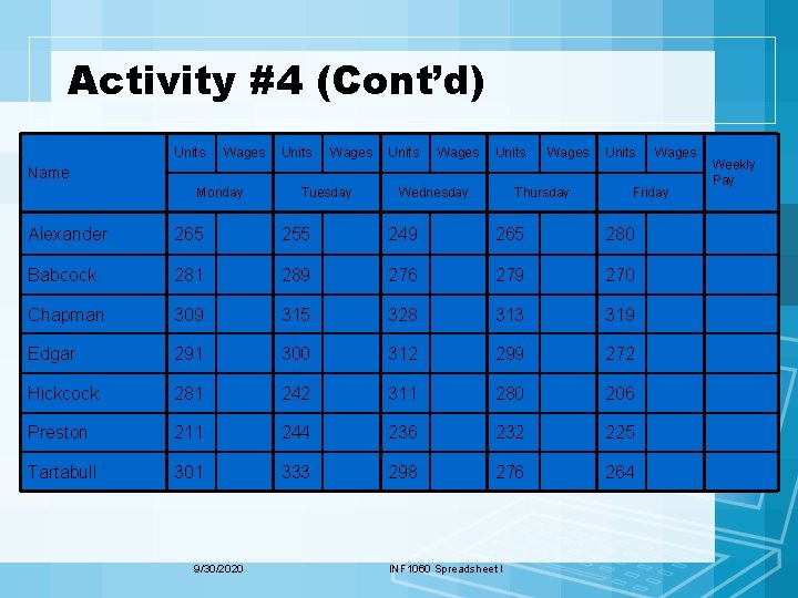
Activity #4 (Cont’d) Units Wages Units Wages Name Monday Tuesday Wednesday Thursday Friday Alexander 265 255 249 265 280 Babcock 281 289 276 279 270 Chapman 309 315 328 313 319 Edgar 291 300 312 299 272 Hickcock 281 242 311 280 206 Preston 211 244 236 232 225 Tartabull 301 333 298 276 264 9/30/2020 INF 1060 Spreadsheet I Weekly Pay

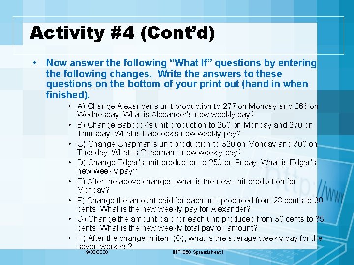
Activity #4 (Cont’d) • Now answer the following “What If” questions by entering the following changes. Write the answers to these questions on the bottom of your print out (hand in when finished). • A) Change Alexander’s unit production to 277 on Monday and 266 on Wednesday. What is Alexander’s new weekly pay? • B) Change Babcock’s unit production to 260 on Monday and 270 on Thursday. What is Babcock’s new weekly pay? • C) Change Chapman’s unit production to 320 on Monday and 300 on Tuesday. What is Chapman’s new weekly pay? • D) Change Edgar’s unit production to 250 on Friday. What is Edgar’s new weekly pay? • E) After the above changes, what is the new unit production for Monday? • F) Change the amount paid for each unit produced from 28 cents to 30 cents. What is the new weekly pay for Alexander? • G) Change the amount paid for each unit produced from 30 cents to 35 cents. What is the new weekly total payroll amount? • H) After the change in item (G), what is the average weekly pay for the seven workers? 9/30/2020 INF 1060 Spreadsheet I

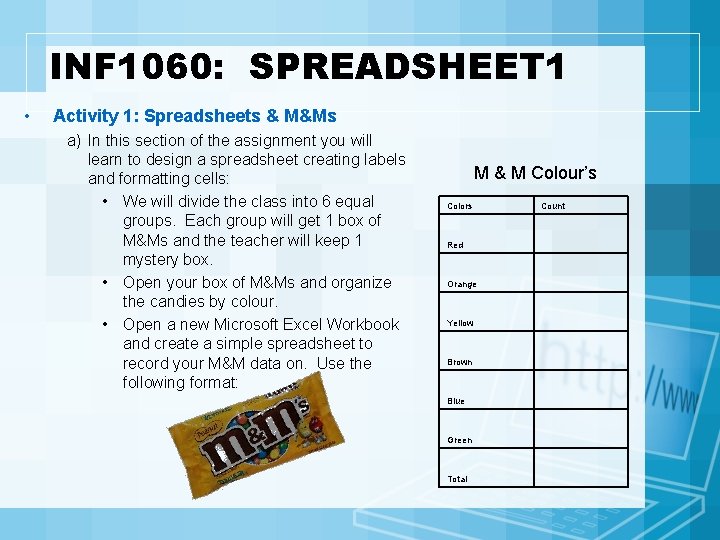
INF 1060: SPREADSHEET 1 • Activity 1: Spreadsheets & M&Ms a) In this section of the assignment you will learn to design a spreadsheet creating labels and formatting cells: • We will divide the class into 6 equal groups. Each group will get 1 box of M&Ms and the teacher will keep 1 mystery box. • Open your box of M&Ms and organize the candies by colour. • Open a new Microsoft Excel Workbook and create a simple spreadsheet to record your M&M data on. Use the following format: M & M Colour’s Colors Red Orange Yellow Brown Blue Green Total Count

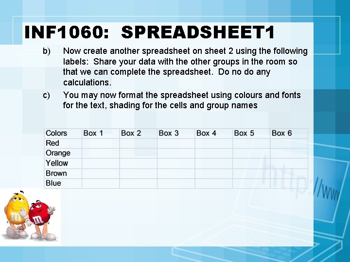
INF 1060: SPREADSHEET 1 b) c) Now create another spreadsheet on sheet 2 using the following labels: Share your data with the other groups in the room so that we can complete the spreadsheet. Do no do any calculations. You may now format the spreadsheet using colours and fonts for the text, shading for the cells and group names

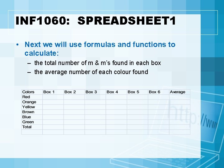
INF 1060: SPREADSHEET 1 • Next we will use formulas and functions to calculate: – the total number of m & m’s found in each box – the average number of each colour found

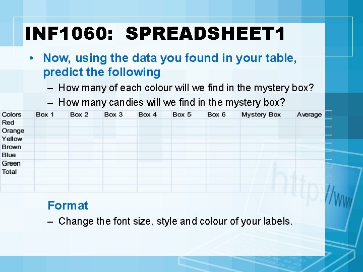
INF 1060: SPREADSHEET 1 • Now, using the data you found in your table, predict the following – How many of each colour will we find in the mystery box? – How many candies will we find in the mystery box? Format – Change the font size, style and colour of your labels.

INF 1060: SPREADSHEET 1 Assignment # 1 Sum Function, formatting cells and adding images • Your new Mc. Donalds job has proved to be very lucrative. In just 6 months, you have saved enough money to buy an i. Pod. • While shopping, you can’t resist buying a few other accessories for your i. Pod (minimum of 10). • Go on the internet and find prices and pictures for the i. Pod you will buy and the accessories you will purchase as well. • Create a Spreadsheet that lists the items you will purchase and the prices for each item. • Format the Spreadsheet by changing fonts, colours shading and borders. Add an image for each of the items that you purchase. • Use the Sum function to find the total cost of the items. • Calculate the GST for these items – use 5% • Find the total cost of your purchase.

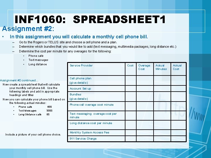
INF 1060: SPREADSHEET 1 Assignment #2: • In this assignment you will calculate a monthly cell phone bill. – – – Go to the Rogers or TELUS site and choose a cell phone and a plan. Determine which bundles that you would like to add (text messaging, multimedia packages, long distance etc. ) Determine the cost per minute for any overages for the following: • Phone calls • Text messages • Long distance Service Provider Cost Overage Actual Cost Assignment #2 continued… Now create a spreadsheet that will calculate your monthly cell phone bill. Use the following labels and add in appropriate headings and titles Now you can calculate your phone bill based on the following actual minutes: • • • Phone calls Text Messages Long Distance calls 600 3000 50 Cell phone plan (give details) Account Set up Bundles (give details) Phone call overage cost minute Text messaging overage cost per minute Long distance cost per minute Include a picture of your cell phone choice. Monthly System Access Fee 911 Service Charge Minutes Cost

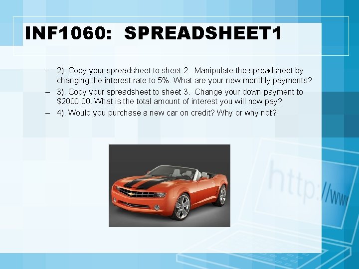
INF 1060: SPREADSHEET 1 Assignment 3 • Your Great Uncle Herbert recently won the lottery and has given you $10000 cash. You decide to use the entire amount as a down payment on a brand new car and take out a loan for the rest of the purchase price. You may purchase any car you wish. (But can you pay for it? ) • 1). Create a spreadsheet that represents the following car loan schedule: • • • Cost of the car GST (5%) Total Cost Less Trade In (if you have one) Less Down Payment Loan Amount Total Interest Payable (10% per year for 4 years) Total Loan Payment Monthly Payments ***Format the spreadsheet with the appropriate formats and add a picture of your car.

INF 1060: SPREADSHEET 1 – 2). Copy your spreadsheet to sheet 2. Manipulate the spreadsheet by changing the interest rate to 5%. What are your new monthly payments? – 3). Copy your spreadsheet to sheet 3. Change your down payment to $2000. What is the total amount of interest you will now pay? – 4). Would you purchase a new car on credit? Why or why not?

Assignment 4 Shopping • Your Grandma just gave • You have the you $2000 for your opportunity to review birthday and is taking your favourite sports you shopping to any team or player’s store you want. statistics • Use Excel to create a spreadsheet of the stores and items you team’s and/ or player’s want to buy. performance. • Be sure to include totals, GST, colour, and totals, averages, colour, gridlines. and gridlines. Sports ** Make sure you look at the guidelines on the next slide**

Guidelines for Assignment 4 q q q q q minimum 3 columns minimum 5 rows minimum of 4 addition or average formulas minimum of 1 multiplication formula appropriate use of merge and center (title) appropriate line spacing (eg. using only one column) only 1 picture (with formatting) use of borders and colour Overall ‘wow factor’ (visual appearance)

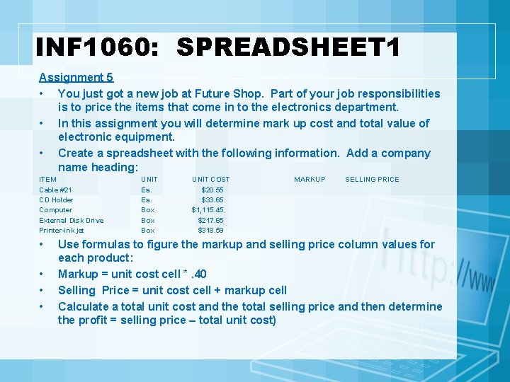
INF 1060: SPREADSHEET 1 Assignment 5 • You just got a new job at Future Shop. Part of your job responsibilities is to price the items that come in to the electronics department. • In this assignment you will determine mark up cost and total value of electronic equipment. • Create a spreadsheet with the following information. Add a company name heading: ITEM Cable #21 CD Holder Computer External Disk Drive Printer-ink jet • • UNIT Ea. Box Box UNIT COST $20. 55 $33. 65 $1, 115. 45 $217. 65 $318. 59 MARKUP SELLING PRICE Use formulas to figure the markup and selling price column values for each product: Markup = unit cost cell *. 40 Selling Price = unit cost cell + markup cell Calculate a total unit cost and the total selling price and then determine the profit = selling price – total unit cost)

Assignment 5. 1 • Go to the following site and watch the video http: //www. youtube. com/watch? v=kh. Wj. Nx 591 rc (DONE) • • • After watching this go into your Assignment 4 (Sports or Shopping) and create a line graph on sheet 2. Add axis titles and gridlines Make sure it is saved to the marking folder in – J: shared/ Info 10/ Brenda and Jen/ Assignment 4

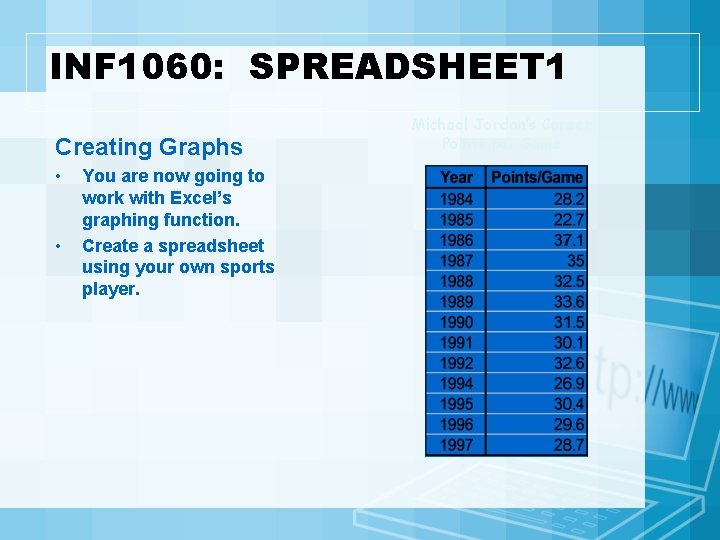
INF 1060: SPREADSHEET 1 Creating Graphs • • You are now going to work with Excel’s graphing function. Create a spreadsheet using your own sports player. Michael Jordan’s Career Points per Game

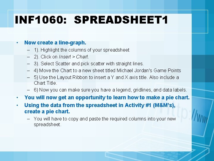
INF 1060: SPREADSHEET 1 • Now create a line-graph. – – – 1). Highlight the columns of your spreadsheet 2). Click on Insert > Chart. 3). Select Scatter and pick scatter with straight lines. 4) Move the Chart to a new sheet titled Michael Jordan's Game Points 5) Use the Layout Ribbon to insert a Y and X axis title. Also include a Chart Title. – 6) Now you can make sure you have a legend, gridlines, and data labels. • • You will now get an opportunity to learn how to make a pie chart. Using the data from the spreadsheet in Activity #1 (M&M’s), create a pie chart. – You will have to copy and paste the required columns into your new spreadsheet.

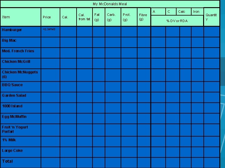
INF 1060: SPREADSHEET 1 Conditional Formatting • Open a spreadsheet and save it to J: shared/ Info 10/ Brenda and Jen/ Assignment 7 Conditional Form. Make sure your file name is “your firstname_yourlastname” • You love eating at Mc. Donald’s. Your parents, on the other hand, think that it is way too unhealthy! You are determined to prove them wrong. So, you set out to create a daily diet that is nutritionally complete, and comprised entirely of food from Mc. Donald’s. • You will create a spreadsheet of selected Mc. Donald’s menu items and use it to determine the nutritional content and price of a number of different “Mc. Meals”!

INF 1060: SPREADSHEET 1 • Create a spreadsheet using the following information. Include titles, labels, values, and formulas. • Apply necessary formatting. • Be sure you use cell references. • **Add a column titled “Quantity” at the end of your spreadsheet. – By manipulating the quantity of each item, your totals should also change (eg. if you change the number of hamburgers to 2, the price and nutritional information in the hamburger ‘row’ will double). • Be sure you put a working hyperlink into your spreadsheet that will take the viewer to the website you got your Mc. Donalds nutrition facts from.

My Mc. Donalds Meal Item Price Hamburger =2. 34*M 3 Big Mac Med. French Fries Chicken Mc. Grill Chicken Mc. Nuggets (6) BBQ Sauce Garden Salad 1000 Island Egg Mc. Muffin Fruit ‘n Yogurt Parfait 1% Milk Large Coke Total Cal. from fat Fat (g) Carb. (g) Prot. (g) Fibre (g) A C Calc % DV or RDA Iron Quantit y

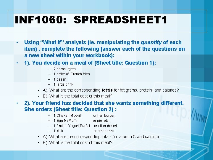
INF 1060: SPREADSHEET 1 • • Using “What If” analysis (ie. manipulating the quantity of each item) , complete the following (answer each of the questions on a new sheet within your workbook): 1). You decide on a meal of (Sheet title: Question 1): – – 2 hamburgers 1 order of French fries 1 desert 1 large drink • A). What are the corresponding totals for fat grams, protein, and calories? • B). What is the total cost of this meal? • 2). Your friend has decided that she wants something different. She orders (Sheet title: Question 2) : – – 1 Chicken Mc. Grill or hamburger 1 Egg Mc. Muffin or pie, etc. 1 Fruit ‘n Yogurt Parfait or other desert 1 Milk or other drink • A). What are the corresponding totals for vitamin C and calcium. • B). What is the total cost of this meal?

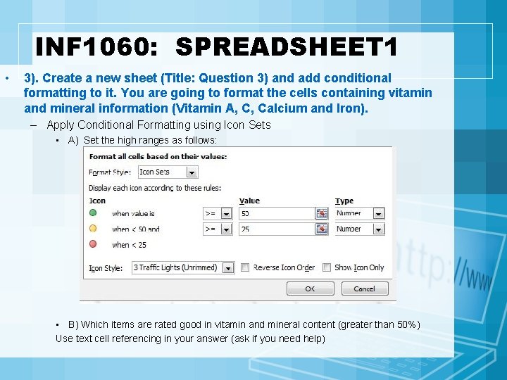
INF 1060: SPREADSHEET 1 • 3). Create a new sheet (Title: Question 3) and add conditional formatting to it. You are going to format the cells containing vitamin and mineral information (Vitamin A, C, Calcium and Iron). – Apply Conditional Formatting using Icon Sets • A) Set the high ranges as follows: • B) Which items are rated good in vitamin and mineral content (greater than 50%) Use text cell referencing in your answer (ask if you need help)

INF 1060: SPREADSHEET 1 • 4). Next, create a diet that ensures you have met both your (Sheet Title: Question 4) – protein (at least 50 g) and – fat (no more than 67 g) requirements. Instructions – Use conditional formatting on the total protein cell to highlight green when protein is greater than or equal to 50 g. – Use conditional formatting on the fat (g) cell to highlight green when fat is less than or equal to 67 g. – Now you must work with your quantities until the total protein and total fat cells turn green. – What is the total cost of this diet?

INF 1060: SPREADSHEET 1 • 5). Design a diet that will prove your parents wrong… you can eat healthy at Mc. Donald’s! – Keep in mind that this diet must meet the following requirements (use conditional formatting on the totals cells to achieve these results): • • Calories have to be as close as possible to 2000 Vitamin A, C, calcium and iron must all be at least 100%. Protein must be greater than 50 Total fat grams must be less than 67 On your spreadsheet answer the following questions: A). What are the menu items that make up your diet? B). How much does your diet cost? C). Based on your experience with “what-if” analysis, briefly outline what you see as the benefits of this kind of analysis. What are the weaknesses? (Use the internet to search answers if you need help, make sure you cite any online information) D). What are some practical applications of this method in the “real-world”?

INF 1060: SPREADSHEET 1 • 6). Go to http: //www. internet 4 classrooms. com/excel _conditional_formatting_07. htm and follow the onscreen directions.

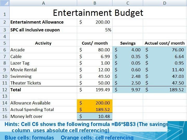
A) Assignment 8 - Absolute Cell Referencing • Choose your own 5 -10 entertainment activities. • On sheet 1 create your spreadsheet and rename the sheet Entertainment 1. • Be sure you sort your activities in alphabetical order using the sort tool before entering your amounts or formulas. • Follow the sample (next slide) to calculate your total savings with a 5% discount and allowance of $200. • Hint: use the dollar sign feature on the drop down menu of the ribbon and the ‘percentage’ option located in the same area.

Hints: Cell C 6 shows the following formula =B 6*$B$3 (The savings column uses absolute cell referencing) Blue cells: formulas Orange cells: cell referencing

B) • Copy and paste your spreadsheet onto sheet 2 • Name this sheet Entertainment 2. • Now change your coupon savings rate to 20% • Add a background. • How much money do you have left now? (write the questions and answer directly on this sheet). C) • Use the sheet Entertainment 2 sheet to create a chart on its own page. Include (axis labels, title, legend, gridlines)

D) • Print Entertainment 1 and 2 in show formulas view. Be sure to put your name in a footer and print to 1 page. • Print your chart. Be sure to put your name in the footer and print to one page. • All 3 printed pages are due at the end of class. • Be sure to also save your assignment in the J: shared Info 10 folder.

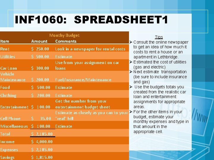
INF 1060: SPREADSHEET 1 Personal Budget • • In this activity, you will create a monthly budget based on income earned from a fictitious job versus estimated living expenses (including rent, transportation, food, and leisure time activities). If your expenses exceed your income, you will need to determine where to cut back your monthly expenses in order to "make ends meet. " You will also encounter unexpected monthly expenses which will force you to adjust your monthly budget.

INF 1060: SPREADSHEET 1 Item Monthy Budget Amount Comments Rent $ 250. 00 Utilities $ 500. 00 Car Loan Vehicle Maintenance $ 300. 00 Food $ 500. 00 Clothing $ 200. 00 Entertainment $ 100. 00 Cell Phone $ 35. 00 Miscellaneous $ 100. 00 Total $ 2, 185. 00 Income $ 4, 000. 00 Expenses $ 2, 185. 00 Savings $ 1, 815. 00 Tips Ø Consult the online newspaper to get an idea of how much it Look in a newspaper for rental costs to rent a house or an Estimate apartment in Lethbridge. Ø Estimated the cost of utilities Use from your assignment on car (gas and electric) loans Ø Next estimate transportation (be sure to include insurance Fuel/Insurance/Maintenance and gas) Ø Use the budgets totals you Estimate created from the realistic car Estimate loan and entertainment Get the number from your assignments for appropriate areas. entertainment budget sheet Estimate as closely as you can to your Ø For the other items in your budget, estimate your "real" bill monthly expenses and type in Estimate that amount in the appropriate cell.

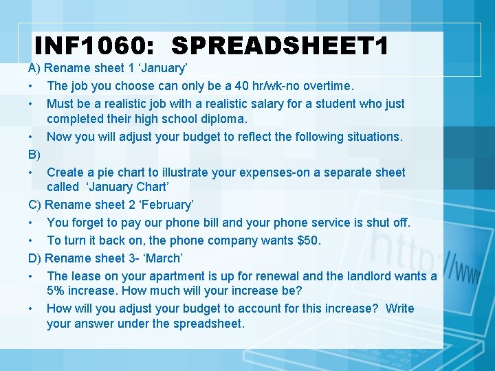
INF 1060: SPREADSHEET 1 A) Rename sheet 1 ‘January’ • The job you choose can only be a 40 hr/wk-no overtime. • Must be a realistic job with a realistic salary for a student who just completed their high school diploma. • Now you will adjust your budget to reflect the following situations. B) • Create a pie chart to illustrate your expenses-on a separate sheet called ‘January Chart’ C) Rename sheet 2 ‘February’ • You forget to pay our phone bill and your phone service is shut off. • To turn it back on, the phone company wants $50. D) Rename sheet 3 - ‘March’ • The lease on your apartment is up for renewal and the landlord wants a 5% increase. How much will your increase be? • How will you adjust your budget to account for this increase? Write your answer under the spreadsheet.

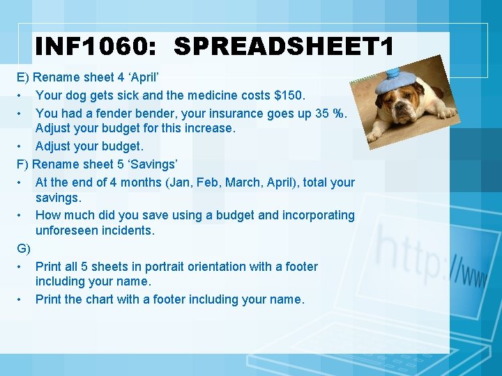
INF 1060: SPREADSHEET 1 E) Rename sheet 4 ‘April’ • Your dog gets sick and the medicine costs $150. • You had a fender bender, your insurance goes up 35 %. Adjust your budget for this increase. • Adjust your budget. F) Rename sheet 5 ‘Savings’ • At the end of 4 months (Jan, Feb, March, April), total your savings. • How much did you save using a budget and incorporating unforeseen incidents. G) • Print all 5 sheets in portrait orientation with a footer including your name. • Print the chart with a footer including your name.

Other Optional Assignments

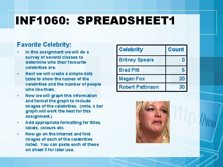
INF 1060: SPREADSHEET 1 Favorite Celebrity: • • • In this assignment we will do a survey of several classes to determine who their favourite celebrities are. Next we will create a simple data table to show the names of the celebrities and the number of people who like them. Now we will graph this information and format the graph to include images of the celebrities. (note, a bar graph will work the best for this assignment. ) Add appropriate formatting for titles, labels, colours etc. Now go on the Internet and find images of each of the celebrities listed. You can paste each of these on sheet 3 for later use. Celebrity Count Britney Spears 0 Brad Pitt 5 Megan Fox 20 Robert Pattinson 30

Now that you have data you will create a bar chart using the chart wizard in Excel: – Select a single bar, or column, on the chart. This requires two clicks. The first click selects all bars, the second click will select a single bar or column. – Go back to the worksheet which contains the image you wish to use. Click on the image to select it, then copy the image. Once the image has been stored in your clipboard return to the chart and paste the image in place of the selected bar or column. – You will see a stretched out mess. Don't worry. Double-click the image to bring up the Format Data Point window. In the image below I cut out part of the window to keep images on this page as small as possible. Select Fill Effects. – On the Picture tab of the Fill Effects window, select the radio button beside Stack and scale to: . Excel will suggest a number of units that each picture will represent. You may change this if you wish. I suggest that you go with the recommended value first, then change if you are not happy with the result. – Select OK twice to get out of this window back to your chart. You will notice that only one bar or column has been changed. – Repeat this process for each of the celebrities photos you want to use.