Inequality Capitalism in the Long Run Thomas Piketty

Inequality & Capitalism in the Long Run Thomas Piketty Paris School of Economics Lindahl Lectures, Part 1, April 24 th 2013

• These lectures: how do wealth-income and inheritanceincome ratios evolve in the long run, and why? • The rise of top income shares will not be covered in these lectures: highly relevant for the US, but less so for Europe • In Europe, and possibly everywhere in the very long run, the key issue the rise of wealth-income ratios and the possible return of inherited wealth • So this lecture will focus on the long run evolution of wealth and inheritance • If you want to know more about top incomes, have a look at « World Top Incomes Database » website

• Key issue today: wealth & inheritance in the long run • There are two ways to become rich: either through one’s own work, or through inheritance • In Ancien Regime societies, as well as in 19 C and early 20 C, it was obvious to everybody that the inheritance channel was important • Inheritance and successors were everywhere in the 19 C literature: Balzac, Jane Austen, etc. • Inheritance flows were huge not only in novels; but also in 19 C tax data: major economic, social and political issue

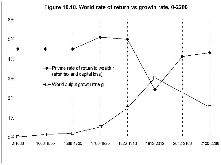
• Question: Does inheritance belong to the past? Did modern growth kill the inheritance channel? E. g. due to the natural rise of human capital and meritocracy? Or due to the rise of life expectancy? • I will answer « NO » to this question: I find that inherited wealth will probably play as big a role in 21 C capitalism as it did in 19 C capitalism • Key mechanism if low growth g and r > g

• An annual inheritance flow around 20%-25% of disposable income is a very large flow • E. g. it is much larger than the annual flow of new savings (typically around 10%-15% of disposable income), which itself comes in part from the return to inheritance (it’s easier to save if you have inherited your house & have no rent to pay) • An annual inheritance flow around 20%-25% of disposable income means that total, cumulated inherited wealth represents the vast majority of aggregate wealth (typically above 80%-90% of aggregate wealth), and vastly dominates self-made wealth

• Main lesson: with g low & r>g, inheritance is bound to dominate new wealth; the past eats up the future g = growth rate of national income and output r = rate of return to wealth = (interest + dividend + rent + profits + capital gains etc. )/(net financial + real estate wealth) • Intuition: with r>g & g low (say r=4%-5% vs g=1%-2%) (=19 C & 21 C), wealth coming from the past is being capitalized faster than growth; heirs just need to save a fraction g/r of the return to inherited wealth • It is only in countries and time periods with g exceptionally high that self-made wealth dominates inherited wealth (Europe in 1950 s-70 s or China today) • r > g & g low might also lead to the return of extreme levels of wealth concentration (not yet: middle class bigger today)

These lectures: three issues (1) The return of wealth (Be careful with « human capital » illusion: human k did not replace non-human financial & real estate capital) (2) The return of inherited wealth (Be careful with « war of ages » illusion: the war of ages did not replace class war; inter-generational inequality did not replace intra-generational inequality) (3) The optimal taxation of wealth & inheritance (With two-dimensional inequality, wealth taxation is useful) (1) : covered in Part 1 (today) (2)-(3) : mostly covered in Part 2 (come back tomorrow!)

• Lectures based upon: • « On the long-run evolution of inheritance: France 18202050 » , QJE 2011 • « Capital is back: wealth-income ratios in rich countries 1700 -2010 » (with Zucman, WP 2013) • « Inherited vs self-made wealth: theory & evidence from a rentier society » (with Postel-Vinay & Rosenthal, 2011) • On-going work on other countries (Atkinson UK, Schinke Germany, Roine-Waldenstrom Sweden, Alvaredo US) → towards a World Wealth & Income Database • « A Theory of Optimal Inheritance Taxation » (with Saez, Econometrica 2013) (all papers are available on line at piketty. pse. ens. fr)

1. The return of wealth • How do aggregate wealth-income ratios evolve in the long-run, and why? • Impossible to address this basic question until recently: national accounts were mostly about flows, not stocks • We compile a new dataset to address this question: - 1970 -2010: Official balance sheets for US, Japan, Germany, France, UK, Italy, Canada, Australia - 1870 -: Historical estimates for US, Germany, France, UK - 1700 -: Historical estimates for France, UK

We Find a Gradual Rise of Private Wealth-National Income Ratios over 1970 -2010 800% 700% 600% USA Japan Germany France UK Italy Canada Australia 500% 400% 300% 200% 1970 1975 1980 1985 1990 1995 2000 2005 Authors' computations using country national accounts. Private wealth = non-financial assets + financial assets - financial liabilities (household & non-profit sectors) 2010

European Wealth-Income Ratios Appear to be Returning to Their High 18 c-19 c Values… 800% 700% 600% Germany France 500% UK 400% 300% 200% 1870 1890 1910 1930 1950 1970 1990 Authors' computations using country national accounts. Private wealth = non-financial assets + financial assets - financial liabilities (household & non-profit sectors) 2010

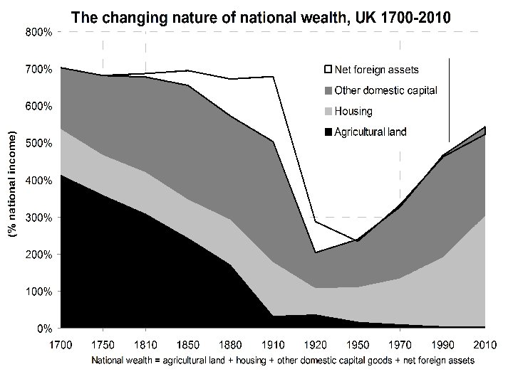
…Despite Considerable Changes in the Nature of Wealth: UK, 1700 -2010 800% Agricultural land 700% Housing Other domestic capital 600% (% national income) Net foreign assets 500% 400% 300% 200% 100% 0% 1700 1750 1810 1850 1880 1910 1920 1950 1970 1990 National wealth = agricultural land + housing + other domestic capital goods + net foreign assets 2010

In the US, the Wealth-Income Ratio Also Followed a U-Shaped Evolution, But Less Marked 800% 700% 600% USA 500% Europe 400% 300% 200% 1870 1890 1910 1930 1950 1970 1990 Authors' computations using country national accounts. Private wealth = non-financial assets + financial assets - financial liabilities (household & non-profit sectors) 2010

What We Are Trying to Understand: The Rise in Private Wealth-National Income Ratios, 1970 -2010 800% 700% 600% USA Japan Germany France UK Italy Canada Australia 500% 400% 300% 200% 1970 1975 1980 1985 1990 1995 2000 2005 Authors' computations using country national accounts. Private wealth = non-financial assets + financial assets - financial liabilities (household & non-profit sectors) 2010

How Can We Explain the 1970 -2010 Evolution? 1. An asset price effect: long run asset price recovery driven by changes in capital policies since world wars 1. A real economic effect: slowdown of productivity and pop growth: – Harrod-Domar-Solow: wealth-income ratio β = s/g – If saving rate s = 10% and growth rate g = 3%, then β ≈ 300% – But if s = 10% and g = 1. 5%, then β ≈ 600% Countries with low g are bound to have high β. Strong effect in Europe, ultimately everywhere.

How Can We Explain Return to 19 c Levels? In very long run, limited role of asset price divergence – In short/medium run, war destructions & valuation effects paramount – But in the very long run, no significant divergence between price of consumption and capital goods – Key long-run force is β = s/g One sector model accounts reasonably well for long run dynamics & level differences Europe vs. US

Three models delivering the same result BU: Bequest-in-utility-function model Max U(c, b)=c 1 -s bs (or Δbs) c = lifetime consumption, b = end-of-life wealth (bequest) s = bequest taste = saving rate → β = s/g DM: Dynastic model: Max Σ U(ct)/(1+δ)t → r = δ +ρg , s = gα/r, β = α/r = s/g ( β ↑ as g ↓) ( U(c)=c 1 -ρ/(1 -ρ) , F(K, L)=KαL 1 -α ) OLG model: low growth implies higher life-cycle savings → in all three models, β = s/g rises as g declines

Growth Rates and Private Saving Rates in Rich Countries, 1970 -2010 Net private Real growth rate saving rate Population rate of per of national (personal + growth rate capita national corporate) income (% national income) U. S. 2. 8% 1. 0% 1. 8% 7. 7% Japan 2. 5% 0. 5% 2. 0% 14. 6% Germany 2. 0% 0. 2% 1. 8% 12. 2% France 2. 2% 0. 5% 1. 7% 11. 1% U. K. 2. 2% 0. 3% 1. 9% 7. 3% Italy 1. 9% 0. 3% 1. 6% 15. 0% Canada 2. 8% 1. 1% 1. 7% 12. 1% Australia 3. 2% 1. 4% 1. 7% 9. 9%

Lesson 1 a: Capital is Back • Low β in mid-20 c were an anomaly – Anti-capital policies depressed asset prices – Unlikely to happen again with free markets – Who owns wealth will become again very important • β can vary a lot between countries – s and g determined by different forces – With perfect markets: scope for very large net foreign asset positions – With imperfect markets: domestic asset price bubbles High β raise new issues about capital regulation & taxation

Private Wealth-National Income Ratios, 1970 -2010, including Spain 800% 700% 600% USA Japan Germany France UK Italy Canada Spain Australia 500% 400% 300% 200% 1970 1975 1980 1985 1990 1995 2000 2005 Authors' computations using country national accounts. Private wealth = non-financial assets + financial assets - financial liabilities (household & non-profit sectors) 2010

From Private to National Wealth: Small and Declining Government Net Wealth, 1970 -2010

National vs. Foreign Wealth, 1970 -2010 (% National Income)

Lesson 1 b: The Changing Nature of Wealth and Technology • In 21 st century: σ > 1 – Rising β come with decline in average return to wealth r – But decline in r smaller than increase in β capital shares α = rβ increase Consistent with K/L elasticity of substitution σ > 1 • In 18 th century: σ < 1 – In 18 c, K = mostly land – In land-scarce Old World, α ≈ 30% – In land-rich New World, α ≈ 15% Consistent with σ < 1: when low substitutability, α large when K relatively scarce

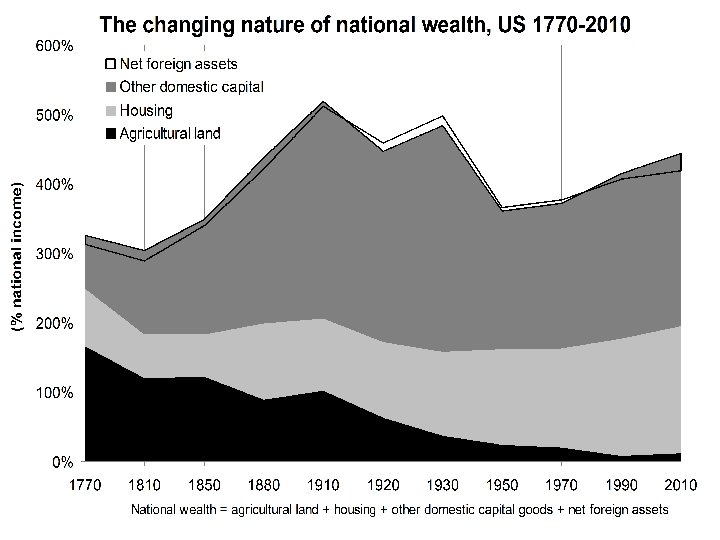
800% The changing nature of national wealth, France 1700 -2010 700% Agricultural land Housing (% national income) 600% Other domestic capital Net foreign assets 500% 400% 300% 200% 100% 0% 1700 1750 1780 1810 1850 1880 1910 1920 1950 1970 1990 2000 National wealth = agricultural land + housing + other domestic capital goods + net foreign assets 2010

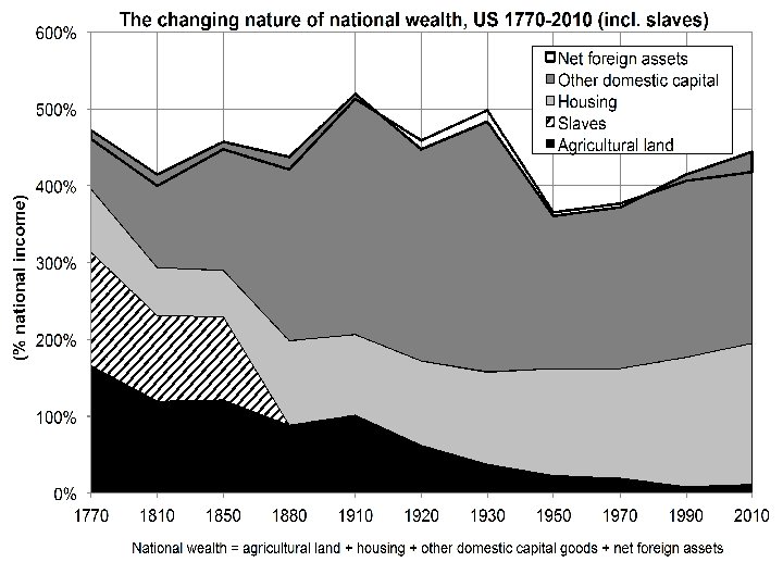
800% National wealth in 1770 -1810: Old vs New world 700% (% national income) 600% Other domestic capital Housing Slaves 500% Agricultural Land 400% 300% 200% 100% 0% UK France US South US North

Rising β Come With Rising Capital Shares α… 40% 35% 30% 25% 20% 15% 10% 1975 1980 1985 1990 USA Japan Germany France UK Canada Australia Italy 1995 2000 2005 2010

… And Slightly Declining Average Returns to Wealth σ > 1 and Finite 12% 10% 8% 6% 4% 2% 0% 1975 1980 USA Japan Germany France UK Canada Australia Italy 1985 1990 1995 2000 2005 2010

End of Part 1: what have we learned? • A world with g low & r>g leads to the return of nonhuman inherited wealth and can be gloomy for workers with zero initial wealth… especially if global tax competition drives capital taxes to 0%… especially if top labor incomes take a rising share of aggregate labor income → A world with g=1. 5% (=long-run world technological frontier? ) is not very different from a world with g=0% (Marx-Ricardo) • From a r-vs-g viewpoint, 21 c maybe not too different from 19 c – but still better than Ancien Regime… except that nobody tried to depict AR as meritocratic…

Inequality & Capitalism in the Long Run Thomas Piketty Paris School of Economics Lindahl Lectures, Part 2, April 25 th 2013

Roadmap of Part 2 (1) The return of wealth (already covered in Part 1; I will just start by presenting a few more technical results) (2) The return of inherited wealth (3) The optimal taxation of wealth & inheritance

1. The Return of Wealth: W & Y Concepts • Wealth – Private wealth W = assets - liabilities of households – Corporations valued at market prices through equities – Government wealth Wg – National wealth Wn = W + Wg – National wealth Wn = K (land + housing + other domestic capital) + NFA (net foreign assets) • Income – Domestic output Yd = F(K, L) (net of depreciation) – National income Y = domestic output Yd + r NFA – Capital share α = rβ (r = average rate of return) β = W/Y = private wealth-national income ratio βn = Wn/Y = national wealth-national income ratio

Accounting for Wealth Accumulation: One Good Model In any one-good model: • At each date t: Wt+1 = Wt + st. Yt → βt+1 = βt (1+gwst)/(1+gt) Ø 1+gwst = 1+st/βt = saving-induced wealth growth rate Ø 1+gt = Yt+1/Yt = output growth rate (productivity + pop. ) • In steady state, with fixed saving rate st=s and growth rate gt=g: βt → β = s/g (Harrod-Domar-Solow formula) Ø Example: if s = 10% and g = 2%, then β = 500%

Accounting for Wealth Accumulation: One Good Model β = s/g is a pure accounting formula, i. e. valid wherever s comes from: • Wealth or bequest in the utility function: saving rate s set by u() (intensity of wealth or bequest taste) and/or demographic structure; β = s/g follows • Dynastic utility: rate of return r set by u(); if α set by technology, then β = α/r follows (s = αg/r, so β = α/r = s/g) • With general utility functions, both s and r are jointly determined by u() and technology

Accounting for Wealth Accumulation: Two Goods Model Two goods: one capital good, one consumption good • Define 1+qt = real rate of capital gain (or loss) = excess of asset price inflation over consumer price inflation • Then βt+1 = βt (1+gwst)(1+qt)/(1+gt) Ø 1+gwst = 1+st/βt = saving-induced wealth growth rate Ø 1+qt = capital-gains-induced wealth growth rate

Our Empirical Strategy • We do not specify where qt come from - maybe stochastic production functions for capital vs. consumption good, with different rates of technical progress • We observe βt, …, βt+n st, …, st+n gt, . . . , gt+n and we decompose the wealth accumulation equation between years t and t + n into: – Volume effect (saving) vs. – Price effect (capital gain or loss)

Data Sources and Method, 1970 -2010 • Official annual balance sheets for top 8 rich countries: – Assets (incl. non produced) and liabilities at market value – Based on census-like methods: reports from financial institutions, housing surveys, etc. – Known issues (e. g. , tax havens) but better than PIM • Extensive decompositions & sensitivity analysis: – – – Private vs. national wealth Domestic capital vs. foreign wealth Private (personal + corporate) vs. personal saving Multiplicative vs. additive decompositions R&D

1970 -2010: A Low Growth and Asset Price Recovery Story • Key results of the 1970 -2010 analysis: – Non-zero capital gains – Account for significant part of 1970 -2010 increase – But significant increase in β would have still occurred without K gains, just because of s & g The rise in β is more than a bubble

What We Are Trying to Understand: The Rise in Private Wealth-National Income Ratios, 1970 -2010 800% 700% 600% USA Japan Germany France UK Italy Canada Australia 500% 400% 300% 200% 1970 1975 1980 1985 1990 1995 2000 2005 Authors' computations using country national accounts. Private wealth = non-financial assets + financial assets - financial liabilities (household & non-profit sectors) 2010

NB: The Rise Would be Even More Spectacular Should We Divide Wealth by Disposable Income 1000% 900% 800% 700% USA Japan Germany France UK Italy Canada Australia 600% 500% 400% 300% 200% 1970 1975 1980 1985 1990 1995 2000 2005 Authors' computations using country national accounts. Private wealth = non-financial assets + financial assets - financial liabilities (household & non-profit sectors) 2010

Growth Rates and Private Saving Rates in Rich Countries, 1970 -2010 Net private Real growth rate saving rate Population rate of per of national (personal + growth rate capita national corporate) income (% national income) U. S. 2. 8% 1. 0% 1. 8% 7. 7% Japan 2. 5% 0. 5% 2. 0% 14. 6% Germany 2. 0% 0. 2% 1. 8% 12. 2% France 2. 2% 0. 5% 1. 7% 11. 1% U. K. 2. 2% 0. 3% 1. 9% 7. 3% Italy 1. 9% 0. 3% 1. 6% 15. 0% Canada 2. 8% 1. 1% 1. 7% 12. 1% Australia 3. 2% 1. 4% 1. 7% 9. 9%

A Pattern of Small, Positive Capital Gains on Private Wealth… U. S. Japan Germany France U. K. Italy Canada Australia Private wealth-national Decomposition of 1970 -2010 wealth growth rate income ratios Real growth Savings. Capital-gainsrate of private induced wealth β (1970) β (2010) wealth growth rate gw gws = s/β q 2. 9% 0. 4% 342% 410% 3. 3% 88% 12% 3. 4% 0. 9% 299% 601% 4. 3% 78% 22% 4. 3% -0. 8% 225% 412% 3. 5% 121% -21% 3. 4% 0. 4% 310% 575% 3. 8% 90% 1. 9% 1. 6% 306% 522% 3. 6% 55% 4. 2% 0. 4% 239% 676% 4. 6% 92% 8% 4. 3% -0. 1% 247% 416% 4. 2% 103% -3% 3. 4% 0. 9% 330% 518% 4. 4% 79% 21%

… But Private Wealth / National Income Ratios Would Have Increased Without K Gains in Low Growth Countries 700% Japan 600% Germany France 500% Italy 400% 300% 200% 1970 1975 1980 1985 1990 1995 2000 2005 Simulated private wealth / national income ratios in the absence of valuation changes, based on 1970 wealth-income ratios, 1970 -2010 private saving flows (including other volume changes) and real income growth rates 2010

From Private to National Wealth: Small and Declining Government Net Wealth, 1970 -2010

Decline in Gov Wealth Means National Wealth Has Been Rising a Bit Less than Private Wealth 900% 800% 700% USA Japan Germany France UK Italy Canada Australia 600% 500% 400% 300% 200% 1970 1975 1980 1985 1990 1995 2000 2005 Authors' computations using country national accounts. National wealth = private wealth + government wealth 2010

National Saving 1970 -2010: Private vs Government Average saving Net national saving rates 1970 -2010 (% (private + national income) government) incl. private saving incl. government saving U. S. 5. 2% 7. 7% -2. 4% Japan 14. 6% 0. 0% Germany 10. 2% 12. 2% -2. 1% France 9. 2% 11. 1% -1. 9% U. K. 5. 3% 7. 3% -2. 0% Italy 8. 5% 15. 0% -6. 5% Canada 10. 1% 12. 1% -2. 0% Australia 8. 9% 9. 9% -0. 9%

Robust Pattern of Positive Capital Gains on National Wealth National wealth-national income ratios β (1970) β (2010) U. S. 404% 431% Japan 359% 616% Germany 313% 416% France 351% 605% U. K. 346% 523% Italy 259% 609% Canada 284% 412% Australia 391% 584% Decomposition of 1970 -2010 wealth growth rate Real growth Savings. Capital-gainsrate of national induced wealth growth rate gw gws = s/β q 2. 1% 0. 8% 3. 0% 72% 28% 3. 1% 0. 8% 3. 9% 78% 22% 3. 1% -0. 4% 2. 7% 114% -14% 2. 7% 0. 9% 3. 6% 75% 25% 1. 8% 3. 3% 45% 55% 2. 6% 1. 5% 4. 1% 63% 37% 3. 4% 0. 4% 3. 8% 89% 11% 2. 5% 1. 6% 4. 2% 61% 39%

Pattern of Positive Capital Gains on National Wealth Largely Robust to Inclusion of R&D

National vs. Foreign Wealth, 1970 -2010 (% National Income)

The Role of Foreign Wealth Accumulation in Rising β U. S. Japan Germany France U. K. Italy Canada Australia National wealth / Rise in national wealth / national income ratio (1970) (2010) (1970 -2010) incl. Foreign Domestic wealth capital 404% 431% 27% 399% 4% 456% -25% 57% -30% 359% 616% 256% 3% 548% 67% 192% 64% 313% 416% 102% 305% 8% 377% 39% 71% 351% 605% 254% 340% 11% 618% -13% 278% -24% 365% 527% 163% 359% 6% 548% -20% 189% -26% 259% 609% 350% 247% 12% 640% -31% 392% -42% 284% 412% 128% 325% -41% 422% -10% 97% 31% 391% 584% 194% 410% -20% 655% -70% 244% -50%

Housing Has Played an Important Role in Many But Not All Countries Domestic capital / national income ratio (1970) U. S. Japan Germany France U. K. Italy Canada Australia Domestic capital / Rise in domestic capital / national income ratio (2010) (1970 -2010) incl. Other incl. Housing domestic capital 399% 456% 57% 142% 257% 182% 274% 41% 17% 356% 548% 192% 131% 225% 220% 328% 89% 103% 305% 377% 71% 129% 177% 241% 136% 112% -41% 340% 618% 278% 104% 236% 371% 247% 267% 11% 359% 548% 189% 98% 261% 300% 248% 202% -13% 247% 640% 392% 107% 141% 386% 254% 279% 113% 325% 422% 97% 108% 217% 208% 213% 101% -4% 410% 655% 244% 172% 239% 364% 291% 193% 52%

2. The return of inherited wealth • In principle, one could very well observe a return of wealth without a return of inherited wealth • I. e. it could be that the rise of aggregate wealthincome ratio is due mostly to the rise of life-cycle wealth (pension funds) • Modigliani life-cycle theory: people save for their old days and die with zero wealth, so that inheritance flows are small

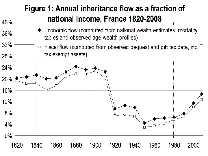
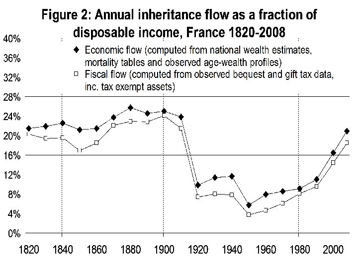
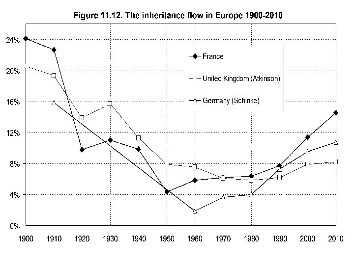
• However the Modigliani story happens to be partly wrong (except in the 1950 s-60 s, when there’s not much left to inherit…): pension wealth is a limited part of wealth (<5% in France… but 20% in the UK) • Bequest flow-national income ratio B/Y = µ m W/Y (with m = mortality rate, µ = relative wealth of decedents) • B/Y has almost returned to 1910 level, both because of W/Y and of µ • Dynastic model: µ = (D-A)/H, m=1/(D-A), so that µ m = 1/H and B/Y = β/H (A = adulthood = 20, H = parenthood = 30, D =death = 60 -80) • General saving model: with g low & r>g, B/Y → β/H → with β=600% & H=generation length=30 years, then B/Y≈20%, i. e. annual inheritance flow ≈ 20% national income

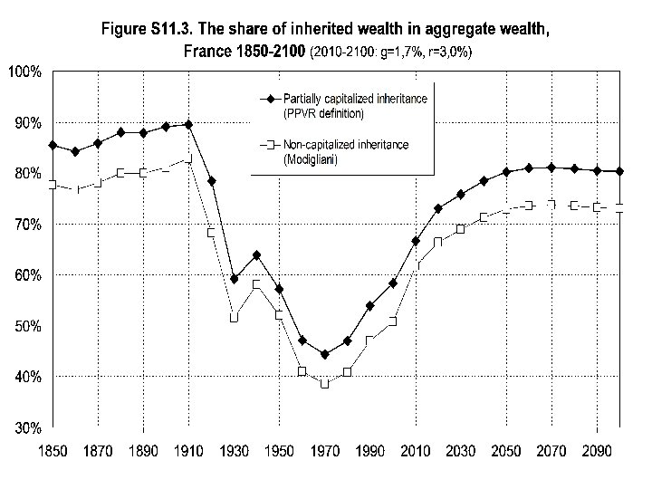
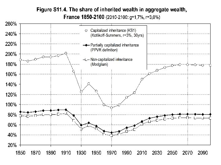
The share of inherited wealth in total wealth • Modigliani AER 1986, JEP 1988: inheritance = 20% of total U. S. wealth • Kotlikoff-Summers JPE 1981, JEP 1988: inheritance = 80% of total U. S. wealth • Three problems with this controversy: - Bad data - We do not live in a stationary world: life-cycle wealth was much more important in the 1950 s-1970 s than it is today - We do not live in a representative-agent world → new definition of inherited share: partially capitalized inheritance (inheritance capitalized in the limit of today’s inheritor wealth) → our findings show that the share of inherited wealth has changed a lot over time, but that it is generally much closer to Kotlikoff-Summers (80%) than Modigliani (20%)

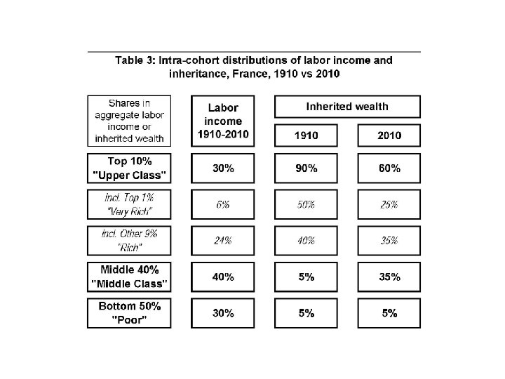
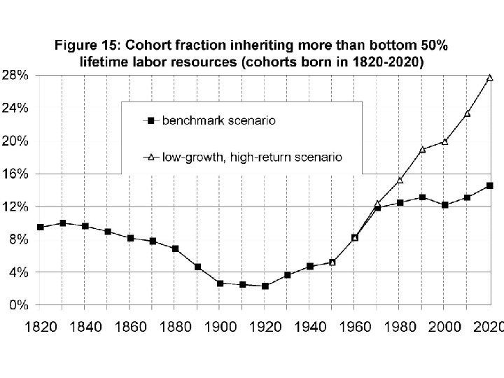
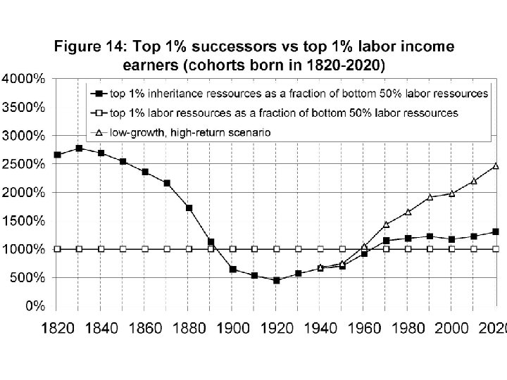
Back to distributional analysis: macro ratios determine who is the dominant social class • 19 C: top successors dominate top labor earners → rentier society (Balzac, Jane Austen, etc. ) • For cohorts born in 1910 s-1950 s, inheritance did not matter too much → labor-based, meritocratic society • But for cohorts born in the 1970 s-1980 s & after, inheritance matters a lot → 21 c class structure will be intermediate between 19 c rentier society than to 20 c meritocratic society – and possibly closer to the former (more unequal in some dimens. , less in others) • The rise of human capital & meritocracy was an illusion. . especially with a labor-based tax system

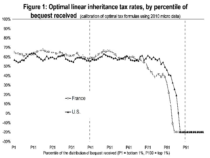
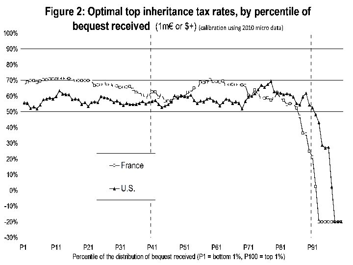
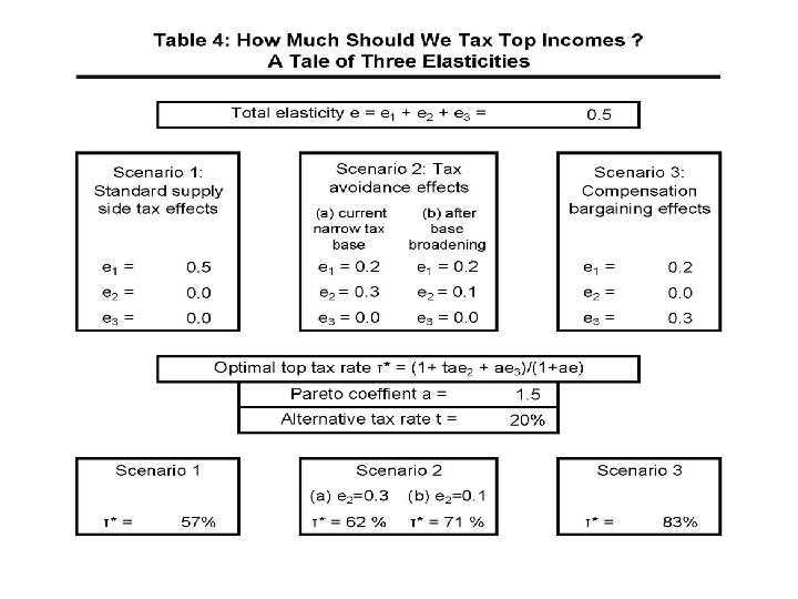
3. The optimal taxation of wealth & inheritance • Summary of main results from Piketty-Saez, « A Theory of Optimal Inheritance Taxation » , Econometrica 2013 • Result 1: Optimal Inheritance Tax Formula (macro version) • Simple formula for optimal bequest tax rate expressed in terms of estimable macro parameters: with: by = macro bequest flow, e. B = elasticity, sb 0 =bequest taste → τB increases with by and decreases with e. B and sb 0 • For realistic parameters: τB=50 -60% (or more. . or less. . . ) → our theory can account for the variety of observed top bequest tax rates (30%-80%)

• Result 2: Optimal Capital Tax Mix • K market imperfections (e. g. uninsurable idiosyncratic shocks to rates of return) can justify shifting one-off inheritance taxation toward lifetime capital taxation (property tax, K income tax, . . ) • Intuition: what matters is capitalized bequest, not raw bequest; but at the time of setting the bequest tax rate, there is a lot of uncertainty about what the rate of return is going to be during the next 30 years → so it is more efficient to split the tax burden → our theory can explain the actual structure & mix of inheritance vs lifetime capital taxation (& why high top inheritance and top capital income tax rates often come together, e. g. US-UK 1930 s-1980 s)

• Meritocratic rawlsian optimum, i. e. social optimum from the viewpoint of zero bequest receivers (z=0): Proposition (zero-receivers tax optimum) with: sb 0 = average bequest taste of zero receivers • τB increases with by and decreases with e. B and sb 0 • If bequest taste sb 0=0, then τB = 1/(1+e. B) → standard revenue-maximizing formula • If e. B →+∞ , then τB → 0 : back to Chamley-Judd • If e. B=0, then τB<1 as long as sb 0>0 • I. e. zero receivers do not want to tax bequests at 100%, because they themselves want to leave bequests → trade-off between taxing rich successors from my cohort vs taxing my own children

Example 1: τ=30%, α=30%, sbo=10%, e. B=0 • If by=20%, then τB=73% & τL=22% • If by=15%, then τB=67% & τL=29% • If by=10%, then τB=55% & τL=35% • If by=5%, then τB=18% & τL=42% → with high bequest flow by, zero receivers want to tax inherited wealth at a higher rate than labor income (73% vs 22%); with low bequest flow they want the oposite (18% vs 42%) Intuition: with low by (high g), not much to gain from taxing bequests, and this is bad for my own children With high by (low g), it’s the opposite: it’s worth taxing bequests, so as to reduce labor taxation and allow zero receivers to leave a bequest

Example 2: τ=30%, α=30%, sbo=10%, by=15% • If e. B=0, then τB=67% & τL=29% • If e. B=0. 2, then τB=56% & τL=31% • If e. B=0. 5, then τB=46% & τL=33% • If e. B=1, then τB=35% & τL=35% → behavioral responses matter but not hugely as long as the elasticity e. B is reasonnable Kopczuk-Slemrod 2001: e. B=0. 2 (US) (French experiments with zero-children savers: e. B=0. 1 -0. 2)

• Optimal Inheritance Tax Formula (micro version) • The formula can be rewritten so as to be based solely upon estimable distributional parameters and upon r vs g : • τB = (1 – Gb*/Ry. L*)/(1+e. B) With: b* = average bequest left by zero-bequest receivers as a fraction of average bequest left y. L* = average labor income earned by zero-bequest receivers as a fraction of average labor income G = generational growth rate, R = generational rate of return • If e. B=0 & G=R, then τB = 1 – b*/y. L* (pure distribution effect) → if b*=0. 5 and y. L*=1, τB = 0. 5 : if zero receivers have same labor income as rest of the pop and expect to leave 50% of average bequest, then it is optimal from their viewpoint to tax bequests at 50% rate • If e. B=0 & b*=y. L*=1, then τB = 1 – G/R (fiscal Golden rule) → if R →+∞, τB → 1: zero receivers want to tax bequest at 100%, even if they plan to leave as much bequest as rest of the pop

What have we learned? (Part 2) • A world with g low & r>g is gloomy for workers with zero initial wealth… especially if global tax competition drives capital taxes to 0%… especially if top labor incomes take a rising share of aggregate labor income • Better integration between empirical & theoretical research is badly needed

Supplementary slides on the evolution of top income shares

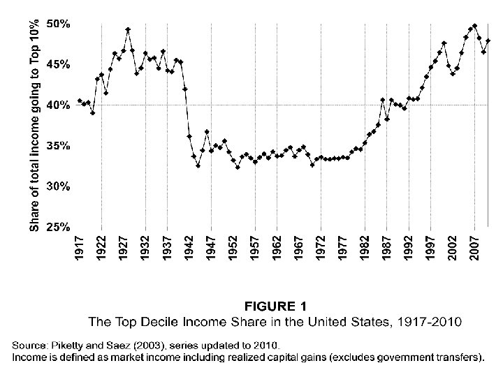
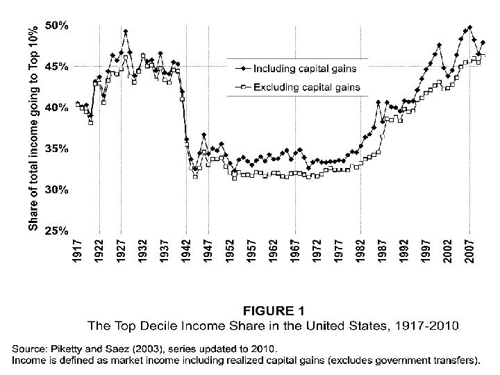
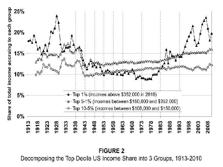
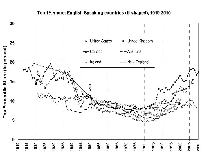
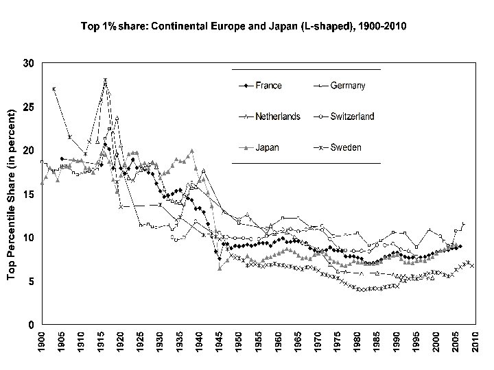
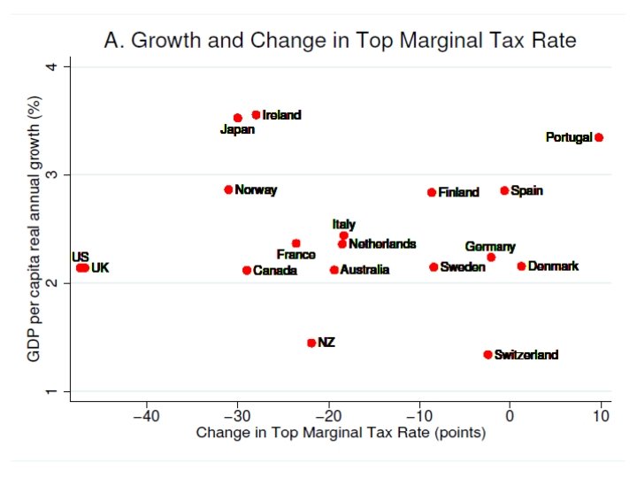
The Continuing Rise of Top Income Shares • World top incomes database: 25 countries, annual series over most of 20 C, largest historical data set • Two main findings: - The fall of rentiers: inequality ↓ during first half of 20 C = top capital incomes hit by 1914 -1945 capital shocks; did not fully recover so far (long lasting shock + progressive taxation) → without war-induced economic & political shock, there would have been no long run decline of inequality; nothing to do with a Kuznets-type spontaneous process - The rise of working rich: inequality ↑ since 1970 s; mostly due to top labor incomes, which rose to unprecedented levels; top wealth & capital incomes also recovering, though less fast; top shares ↓ ’ 08 -09, but ↑ ’ 10; Great Recession is unlikely to reverse the long run trend → what happened?

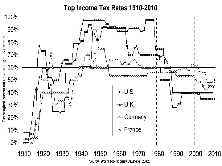
How much should we use progressive taxation to reverse the trend? • Hard to account for observed cross-country variations with a pure technological, marginal-product story • One popular view: US today = working rich get their marginal product (globalization, superstars); Europe today (& US 1970 s) = market prices for high skills are distorted downwards (social norms, etc. ) → very naïve view of the top end labor market & very ideological: we have zero evidence on the marginal product of top executives; it may well be that prices are distorted upwards (more natural for price setters to bias their own price upwards rather than downwards)

• A more realistic view: grabbing hand model = marginal products are unobservable; top executives have an obvious incentive to convince shareholders & subordinates that they are worth a lot; no market convergence because constantly changing corporate & job structure (& costs of experimentation → competition not enough to converge to full information) → when pay setters set their own pay, there’s no limit to rent extraction. . . unless confiscatory tax rates at the very top (memo: US top tax rate (1 m$+) 1932 -1980 = 82%) (no more fringe benefits than today) → see Piketty-Saez-Stantcheva, « Optimal Taxation of Top Labor Incomes » , AEJ-EP 2013 (macro & micro evidence on rising CEO pay for luck)

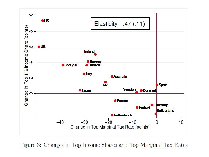
Optimal Taxation of Top Labor Incomes • Standard optimal top tax rate formula: τ = 1/(1+ae) With: e = elasticity of labor supply, a = Pareto coefficient • τ ↓ as elasticity e ↑ : don’t tax elastic tax base • τ ↑ as inequality ↑, i. e. as Pareto coefficient a ↓ (US: a≈3 in 1970 s → ≈1. 5 in 2010 s; b=a/(a-1)≈1. 5 → ≈3) (memo: b = E(y|y>y 0)/y 0 = measures fatness of the top) • Augmented formula: τ = (1+tae 2+ae 3)/(1+ae) With e = e 1 + e 2 + e 3 = labor supply elasticity + income shifting elasticity + bargaining elasticity (rent extraction) • Key point: τ ↑ as elasticity e 3 ↑