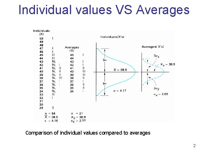
Individual values VS Averages Comparison of individual values

Individual values VS Averages Comparison of individual values compared to averages 2

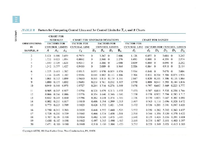
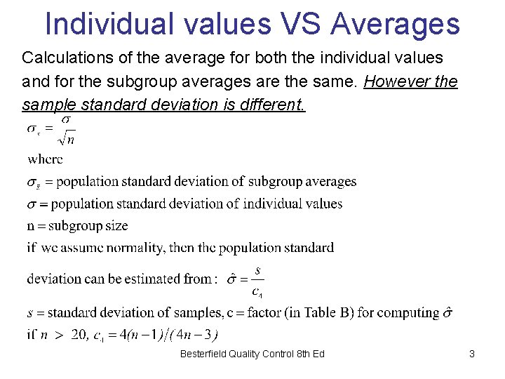
Individual values VS Averages Calculations of the average for both the individual values and for the subgroup averages are the same. However the sample standard deviation is different. Besterfield Quality Control 8 th Ed 3

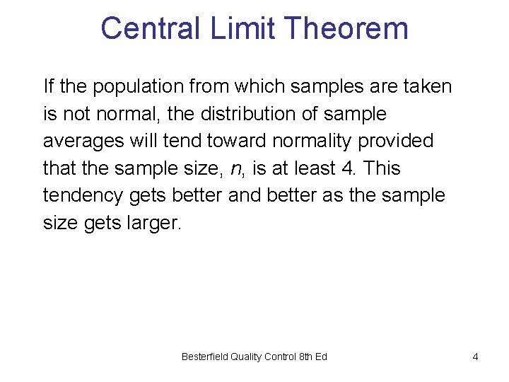
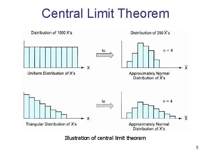
Central Limit Theorem If the population from which samples are taken is not normal, the distribution of sample averages will tend toward normality provided that the sample size, n, is at least 4. This tendency gets better and better as the sample size gets larger. Besterfield Quality Control 8 th Ed 4

Central Limit Theorem Illustration of central limit theorem 5

Central Limit Theorem Dice illustration of central limit theorem Besterfield Quality Control 8 th Ed 6

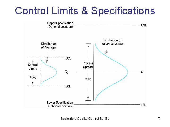
Control Limits & Specifications Figure 5 -21 Relationship of limits, specifications, and distributions Besterfield Quality Control 8 th Ed 7

Control Limits & Specifications q The control limits are established as a function of the average )คา control limits เปนคาทคำนวนจากคาเฉลยทไดจากการเกบขอมล ) q Specifications are the permissible variation in the size of the part and are, therefore, for individual values) คา Specifications เปนคาทกำหนดขนเพอใชเปนขอบเขตของการกระจายสำ หรบคาของขอมลแตละตว ( q The specifications or tolerance limits are established by design engineers or customers Besterfield Quality Control 8 th Ed to meet a particular function 8

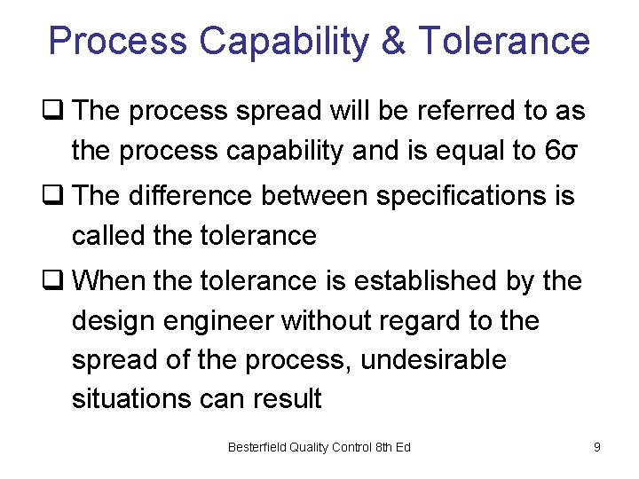
Process Capability & Tolerance q The process spread will be referred to as the process capability and is equal to 6σ q The difference between specifications is called the tolerance q When the tolerance is established by the design engineer without regard to the spread of the process, undesirable situations can result Besterfield Quality Control 8 th Ed 9

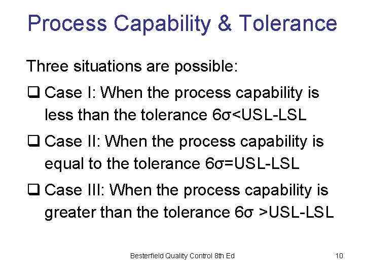
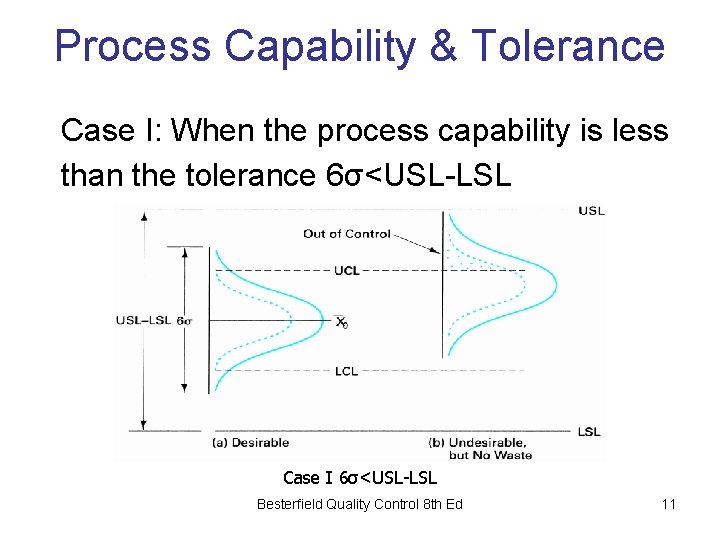
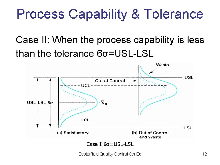
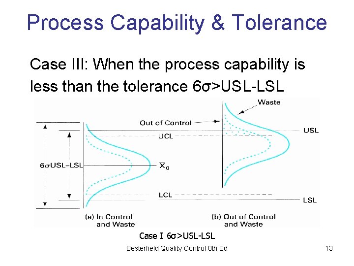
Process Capability & Tolerance Three situations are possible: q Case I: When the process capability is less than the tolerance 6σ<USL-LSL q Case II: When the process capability is equal to the tolerance 6σ=USL-LSL q Case III: When the process capability is greater than the tolerance 6σ >USL-LSL Besterfield Quality Control 8 th Ed 10

Process Capability & Tolerance Case I: When the process capability is less than the tolerance 6σ<USL-LSL Case I 6σ<USL-LSL Besterfield Quality Control 8 th Ed 11

Process Capability & Tolerance Case II: When the process capability is less than the tolerance 6σ=USL-LSL Case I 6σ=USL-LSL Besterfield Quality Control 8 th Ed 12

Process Capability & Tolerance Case III: When the process capability is less than the tolerance 6σ>USL-LSL Case I 6σ>USL-LSL Besterfield Quality Control 8 th Ed 13

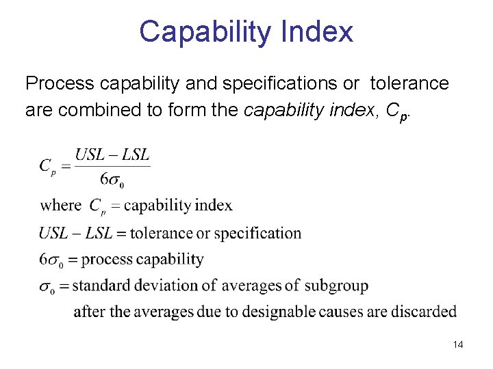
Capability Index Process capability and specifications or tolerance are combined to form the capability index, Cp. 14

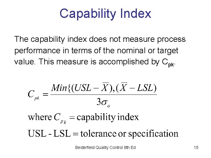
Capability Index The capability index does not measure process performance in terms of the nominal or target value. This measure is accomplished by Cpk. Besterfield Quality Control 8 th Ed 15

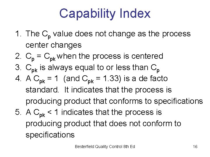
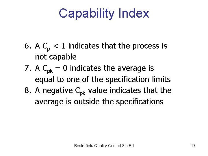
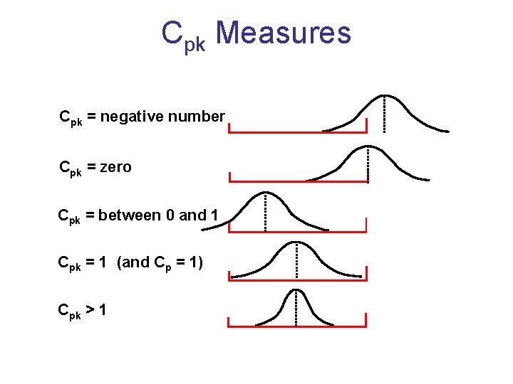
Capability Index 1. The Cp value does not change as the process center changes 2. Cp = Cpk when the process is centered 3. Cpk is always equal to or less than Cp 4. A Cpk = 1 (and Cpk = 1. 33) is a de facto standard. It indicates that the process is producing product that conforms to specifications 5. A Cpk < 1 indicates that the process is producing product that does not conform to specifications Besterfield Quality Control 8 th Ed 16

Capability Index 6. A Cp < 1 indicates that the process is not capable 7. A Cpk = 0 indicates the average is equal to one of the specification limits 8. A negative Cpk value indicates that the average is outside the specifications Besterfield Quality Control 8 th Ed 17

Cpk Measures Cpk = negative number Cpk = zero Cpk = between 0 and 1 Cpk = 1 (and Cp = 1) Cpk > 1

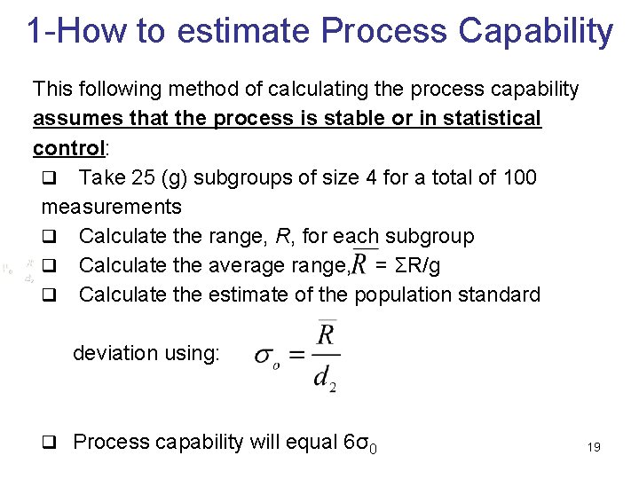
1 -How to estimate Process Capability This following method of calculating the process capability assumes that the process is stable or in statistical control: q Take 25 (g) subgroups of size 4 for a total of 100 measurements q Calculate the range, R, for each subgroup q Calculate the average range, = ΣR/g q Calculate the estimate of the population standard deviation using: q Process capability will equal 6σ0 19

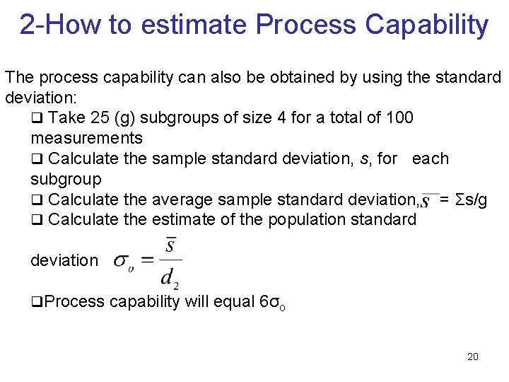
2 -How to estimate Process Capability The process capability can also be obtained by using the standard deviation: q Take 25 (g) subgroups of size 4 for a total of 100 measurements q Calculate the sample standard deviation, s, for each subgroup q Calculate the average sample standard deviation, = Σs/g q Calculate the estimate of the population standard deviation q. Process capability will equal 6σo 20

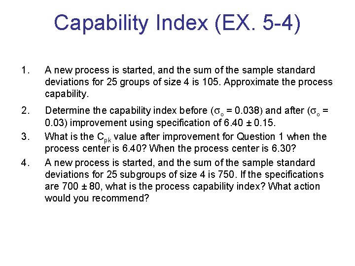
Capability Index (EX. 5 -4) 1. A new process is started, and the sum of the sample standard deviations for 25 groups of size 4 is 105. Approximate the process capability. 2. Determine the capability index before (σo = 0. 038) and after (σo = 0. 03) improvement using specification of 6. 40 ± 0. 15. What is the Cpk value after improvement for Question 1 when the process center is 6. 40? When the process center is 6. 30? A new process is started, and the sum of the sample standard deviations for 25 subgroups of size 4 is 750. If the specifications are 700 ± 80, what is the process capability index? What action would you recommend? 3. 4.

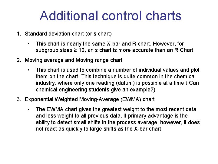
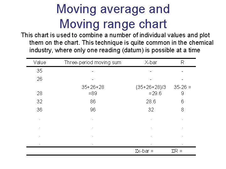
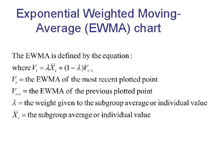
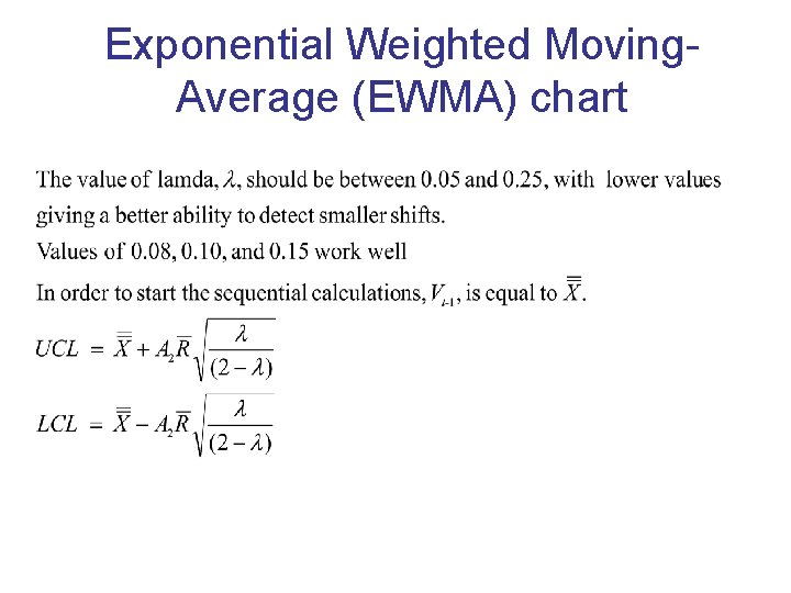
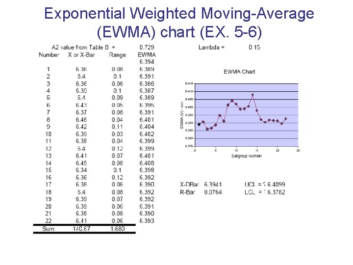
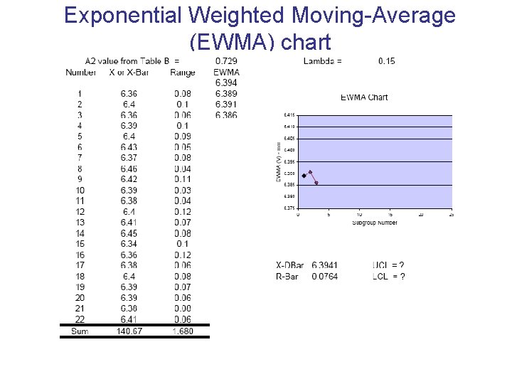
Additional control charts 1. Standard deviation chart (or s chart) • This chart is nearly the same X-bar and R chart. However, for subgroup sizes ≥ 10, an s chart is more accurate than an R Chart 2. Moving average and Moving range chart • This chart is used to combine a number of individual values and plot them on the chart. This technique is quite common in the chemical industry, where only one reading (datum) is possible at a time ( Can chemical engineering students give an example? ) 3. Exponential Weighted Moving-Average (EWMA) chart • The EWMA chart gives the greatest weight to the most recent data and less weight to all previous data. It primary advantage is the ability to detect small shifts in the process average; however, it does not react as quickly to large shifts as the X-bar chart.

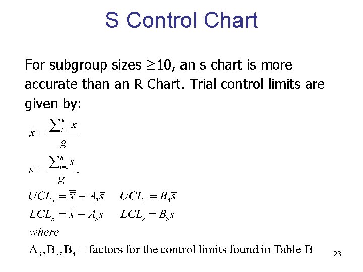
S Control Chart For subgroup sizes ≥ 10, an s chart is more accurate than an R Chart. Trial control limits are given by: 23

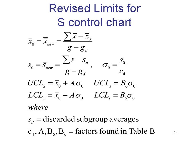
Revised Limits for S control chart 24

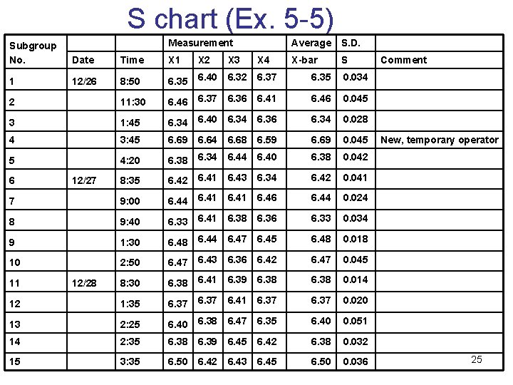
S chart (Ex. 5 -5) Measurement Average S. D. X-bar S Subgroup No. Date Time X 1 X 2 X 3 X 4 1 12/26 8: 50 6. 35 6. 40 6. 32 6. 37 6. 35 0. 034 2 11: 30 6. 46 6. 37 6. 36 6. 41 6. 46 0. 045 3 1: 45 6. 34 6. 40 6. 34 6. 36 6. 34 0. 028 4 3: 45 6. 69 6. 64 6. 68 6. 59 6. 69 0. 045 5 4: 20 6. 38 6. 34 6. 40 6. 38 0. 042 8: 35 6. 42 6. 41 6. 43 6. 34 6. 42 0. 041 7 9: 00 6. 44 6. 41 6. 46 6. 44 0. 024 8 9: 40 6. 33 6. 41 6. 38 6. 36 6. 33 0. 034 9 1: 30 6. 48 6. 44 6. 47 6. 45 6. 48 0. 018 10 2: 50 6. 47 6. 43 6. 36 6. 42 6. 47 0. 045 8: 30 6. 38 6. 41 6. 39 6. 38 0. 014 12 1: 35 6. 37 6. 41 6. 37 0. 020 13 2: 25 6. 40 6. 38 6. 47 6. 35 6. 40 0. 051 14 2: 35 6. 38 6. 39 6. 45 6. 42 6. 38 0. 032 15 3: 35 6. 50 6. 42 6. 43 6. 45 6. 50 0. 036 6 11 12/27 12/28 Comment New, temporary operator 25

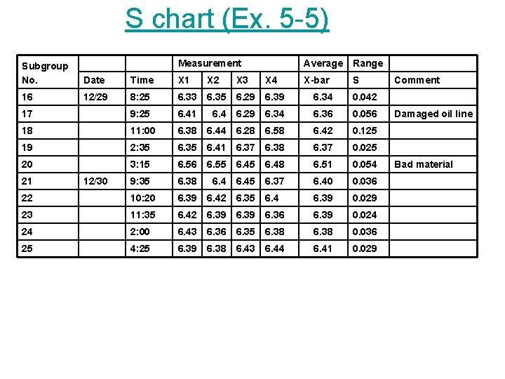
S chart (Ex. 5 -5) Measurement Average Range X-bar S Subgroup No. Date Time X 1 X 2 X 3 X 4 16 12/29 8: 25 6. 33 6. 35 6. 29 6. 34 0. 042 17 9: 25 6. 41 6. 4 6. 29 6. 34 6. 36 0. 056 18 11: 00 6. 38 6. 44 6. 28 6. 58 6. 42 0. 125 19 2: 35 6. 41 6. 37 6. 38 6. 37 0. 025 20 3: 15 6. 56 6. 55 6. 48 6. 51 0. 054 9: 35 6. 38 6. 45 6. 37 6. 40 0. 036 22 10: 20 6. 39 6. 42 6. 35 6. 4 6. 39 0. 029 23 11: 35 6. 42 6. 39 6. 36 6. 39 0. 024 24 2: 00 6. 43 6. 36 6. 35 6. 38 0. 036 25 4: 25 6. 39 6. 38 6. 43 6. 44 6. 41 0. 029 21 12/30 Comment Damaged oil line Bad material

Moving average and Moving range chart This chart is used to combine a number of individual values and plot them on the chart. This technique is quite common in the chemical industry, where only one reading (datum) is possible at a time Value Three-period moving sum X-bar R 35 - - - 26 - - - 28 35+26+28 =89 (35+26+28)/3 =29. 6 35 -26 = 9 32 86 28. 6 6 36 96 32 8 . . . . Sx-bar = SR =

Exponential Weighted Moving. Average (EWMA) chart

Exponential Weighted Moving. Average (EWMA) chart

Exponential Weighted Moving-Average (EWMA) chart (EX. 5 -6)

Exponential Weighted Moving-Average (EWMA) chart

Quiz 5 -1

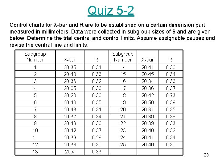
Quiz 5 -2 Control charts for X-bar and R are to be established on a certain dimension part, measured in millimeters. Data were collected in subgroup sizes of 6 and are given below. Determine the trial central and control limits. Assume assignable causes and revise the central line and limits. Subgroup Number X-bar R 1 2 3 4 5 6 7 8 9 10 11 12 13 20. 35 20. 40 20. 36 20. 65 20. 20 20. 43 20. 37 20. 48 20. 42 20. 39 20. 38 20. 4 0. 36 0. 32 0. 36 0. 35 0. 31 0. 34 0. 30 0. 37 0. 29 0. 30 0. 33 Subgroup Number X-bar R 14 15 16 17 18 19 20 21 22 23 24 25 20. 41 20. 45 20. 34 20. 36 20. 42 20. 50 20. 31 20. 39 20. 40 20. 41 20. 40 0. 36 0. 34 0. 36 0. 37 0. 73 0. 38 0. 35 0. 38 0. 33 0. 32 0. 34 0. 30 33

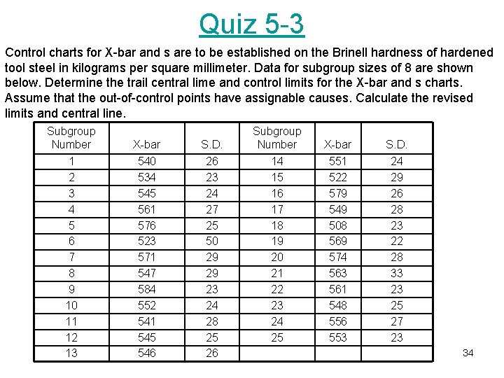
Quiz 5 -3 Control charts for X-bar and s are to be established on the Brinell hardness of hardened tool steel in kilograms per square millimeter. Data for subgroup sizes of 8 are shown below. Determine the trail central lime and control limits for the X-bar and s charts. Assume that the out-of-control points have assignable causes. Calculate the revised limits and central line. Subgroup Number 1 2 3 4 5 6 7 8 9 10 11 12 13 X-bar 540 534 545 561 576 523 571 547 584 552 541 545 546 S. D. 26 23 24 27 25 50 29 29 23 24 28 25 26 Subgroup Number 14 15 16 17 18 19 20 21 22 23 24 25 X-bar 551 522 579 549 508 569 574 563 561 548 556 553 S. D. 24 29 26 28 23 22 28 33 23 25 27 23 34

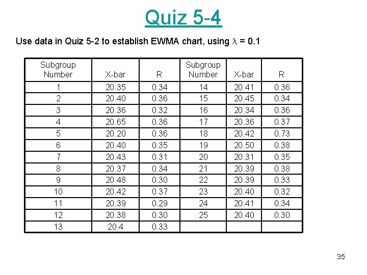
Quiz 5 -4 Use data in Quiz 5 -2 to establish EWMA chart, using = 0. 1 Subgroup Number X-bar R 1 2 3 4 5 6 7 8 9 10 11 12 13 20. 35 20. 40 20. 36 20. 65 20. 20 20. 43 20. 37 20. 48 20. 42 20. 39 20. 38 20. 4 0. 36 0. 32 0. 36 0. 35 0. 31 0. 34 0. 30 0. 37 0. 29 0. 30 0. 33 Subgroup Number X-bar R 14 15 16 17 18 19 20 21 22 23 24 25 20. 41 20. 45 20. 34 20. 36 20. 42 20. 50 20. 31 20. 39 20. 40 20. 41 20. 40 0. 36 0. 34 0. 36 0. 37 0. 73 0. 38 0. 35 0. 38 0. 33 0. 32 0. 34 0. 30 35