INDIRECT METHODS FOR SOLVING SYSTEMS OF LINEAR EQUATIONS

INDIRECT METHODS FOR SOLVING SYSTEMS OF LINEAR EQUATIONS

ITERATIVE METHODS • The preceding methods of solving the system of simultaneous algebraic linear equations are direct methods, as these methods yield the solution after a certain amount of fixed computation. • On the other hand, an iterative method is that in which we start from an approximation to the true solution and obtain better and better approximations from a repeated computation as often as may be necessary for achieving a desired accuracy.

CONT’D • Thus in an iterative method, the number of iterations depends on the degree of accuracy required and the initial solution. • This iterative method is not always successful to all systems of equations. • If this method is to succeed, each equation of the system must possess one large coefficient and the large coefficient must be attached to a different unknown in that equation.

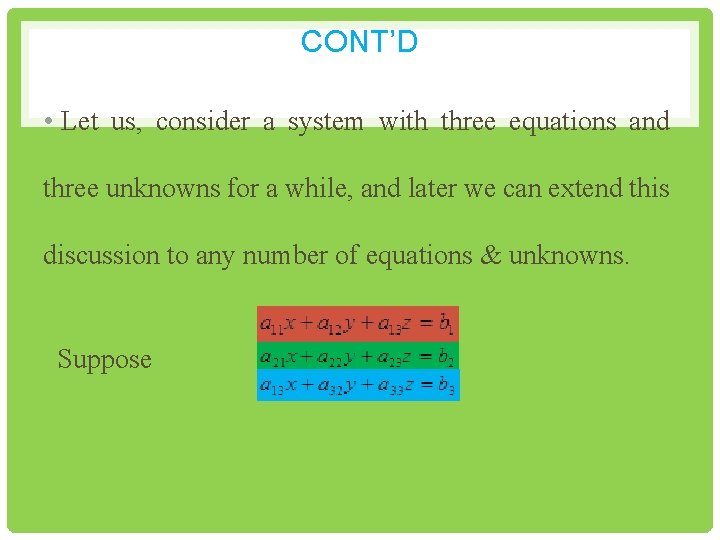
CONT’D • Let us, consider a system with three equations and three unknowns for a while, and later we can extend this discussion to any number of equations & unknowns. Suppose

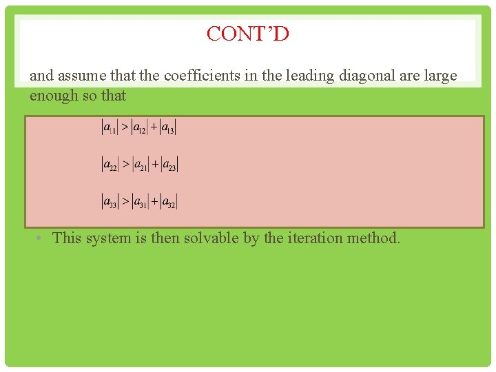
CONT’D and assume that the coefficients in the leading diagonal are large enough so that • This system is then solvable by the iteration method.

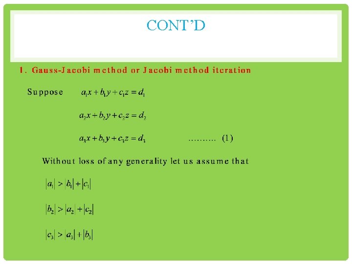
CONT’D • In other words, the solution exists (iteration will converge) if the absolute values of the leading diagonal elements of the coefficient matrix A of the system Ax = B are greater than the sum of absolute values of the other coefficients of the row. We say such a matrix A, a diagonally dominant matrix. • Notice that the condition is sufficient but not necessary.

CONT’D

CONT’D

CON’T

CONT’D

CONT’D

CONT’D

CONT’D

CONT’D

CONT’D

CONT’D

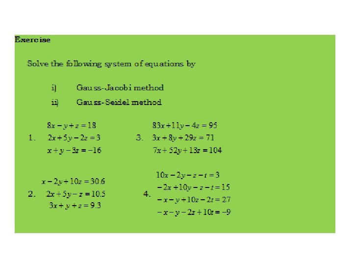
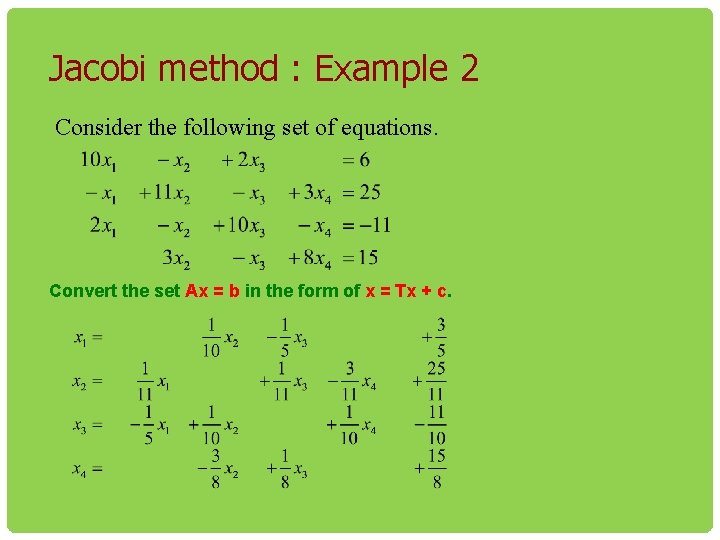
Jacobi method : Example 2 Consider the following set of equations. Convert the set Ax = b in the form of x = Tx + c.

Jacobi method : Example 2

Jacobi method : Example 2

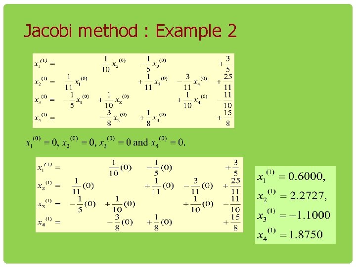
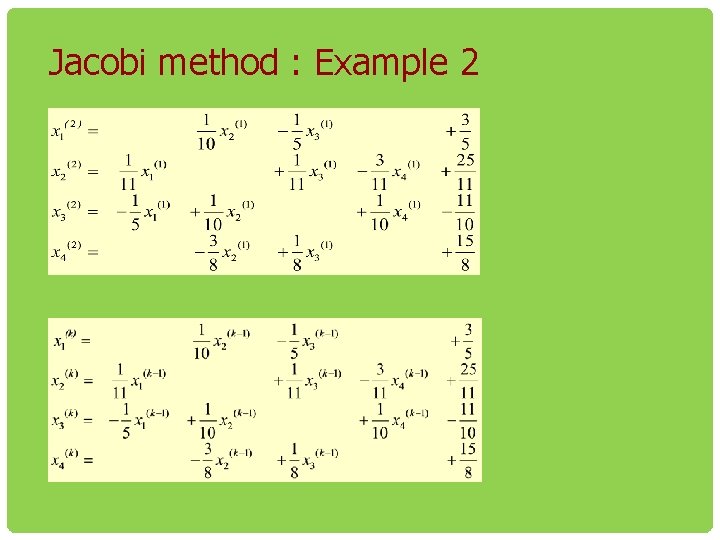
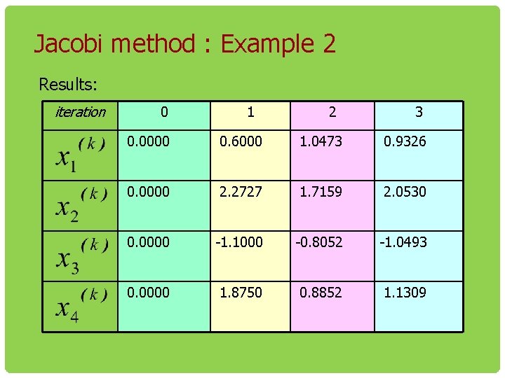
Jacobi method : Example 2 Results: iteration 0 1 2 3 0. 0000 0. 6000 1. 0473 0. 9326 0. 0000 2. 2727 1. 7159 2. 0530 0. 0000 -1. 1000 -0. 8052 -1. 0493 0. 0000 1. 8750 0. 8852 1. 1309

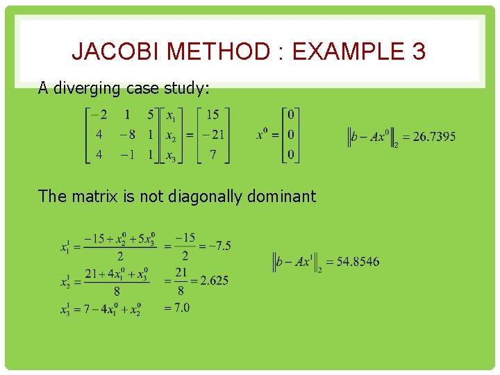
JACOBI METHOD : EXAMPLE 3 A diverging case study: The matrix is not diagonally dominant

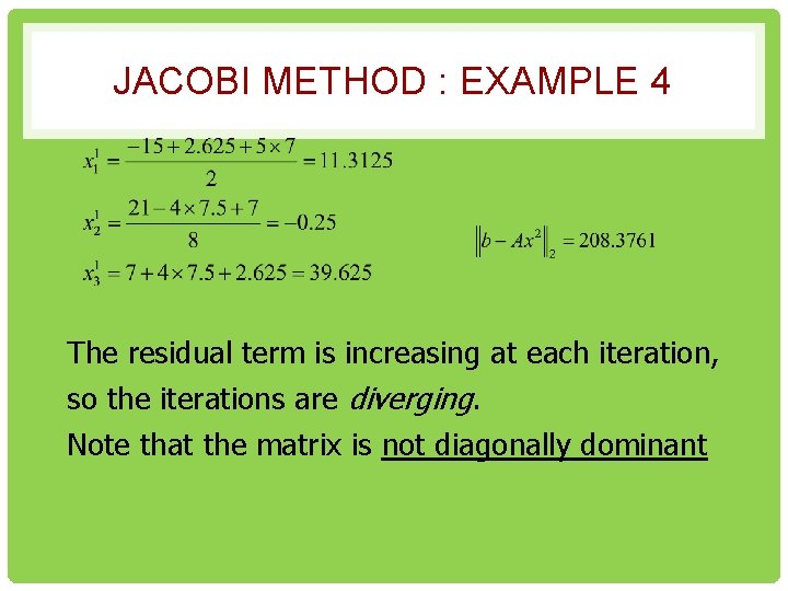
JACOBI METHOD : EXAMPLE 4 The residual term is increasing at each iteration, so the iterations are diverging. Note that the matrix is not diagonally dominant

2. GAUSS-SEIDEL ITERATION METHOD

CONT’D

CONT’D

CONT’D

CONT’D

CONT’D

CONT’D

CONT’D

CONT’D

GAUSS-SEIDEL METHOD: EXAMPLE 2 Given the system of equations The coefficient matrix is: With an initial guess of Will the solution converge using the Gauss-Siedel method?

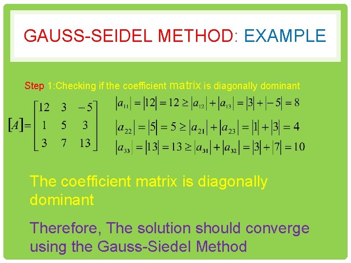
GAUSS-SEIDEL METHOD: EXAMPLE Step 1: Checking if the coefficient matrix is diagonally dominant Therefore, The solution should converge using the Gauss-Siedel Method

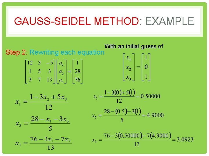
GAUSS-SEIDEL METHOD: EXAMPLE Step 2: Rewriting each equation With an initial guess of

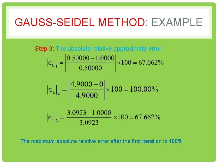
GAUSS-SEIDEL METHOD: EXAMPLE Step 3: The absolute relative approximate error The maximum absolute relative error after the first iteration is 100%

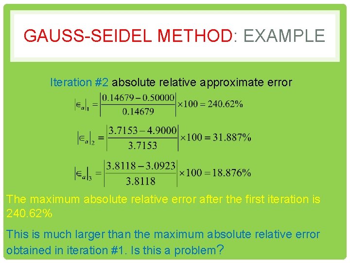
GAUSS-SEIDEL METHOD: EXAMPLE Iteration #2 absolute relative approximate error The maximum absolute relative error after the first iteration is 240. 62% This is much larger than the maximum absolute relative error obtained in iteration #1. Is this a problem?

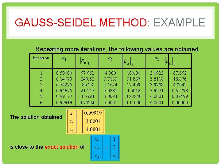
GAUSS-SEIDEL METHOD: EXAMPLE Repeating more iterations, the following values are obtained Iteration a 1 1 2 3 4 5 6 0. 50000 0. 14679 0. 74275 0. 94675 0. 99177 0. 99919 a 2 67. 662 240. 62 80. 23 21. 547 4. 5394 0. 74260 The solution obtained is close to the exact solution of 4. 900 3. 7153 3. 1644 3. 0281 3. 0034 3. 0001 a 3 100. 00 31. 887 17. 409 4. 5012 0. 82240 0. 11000 3. 0923 3. 8118 3. 9708 3. 9971 4. 0001 67. 662 18. 876 4. 0042 0. 65798 0. 07499 0. 00000