Indexing Multidimensional Feature Spaces Overview of Multidimensional Index

Indexing Multidimensional Feature Spaces Overview of Multidimensional Index Structure Hybrid Tree, Chakrabarti et. al. ICDE 1999 Local Dimensionality Reduction, Chakrabarti et. al. VLDB 2000

Queries over Feature Spaces • Consider a d-dimensional feature space – color histogram, texture, … • Nature of Queries – range queries: objects that reside within the region specified in the query – K-nearest neighbor queries: objects that are closest to a query object based on a distance metric – Approx. nearest neighbor queries: retrieved object is within (1+ epsilon) of the real nearest neighbor. – All-pair (similarity join) queries: retrieve all pairs of objects within a epsilon threshold. • A search algorithm may include: – false positives: objects that do not meet the query condition, but are retrieved anyway. We tend to minimize false positives – false negatives: objects that meet the query condition but are not returned. Usually, approaches avoid false negatives

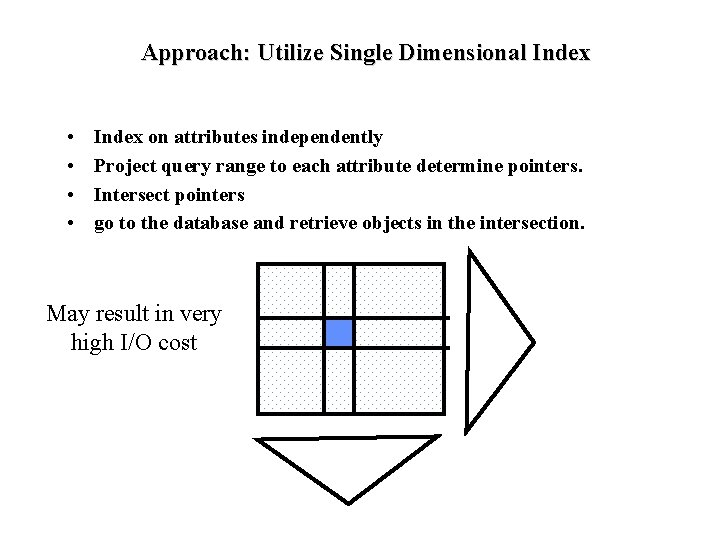
Approach: Utilize Single Dimensional Index • • Index on attributes independently Project query range to each attribute determine pointers. Intersect pointers go to the database and retrieve objects in the intersection. May result in very high I/O cost

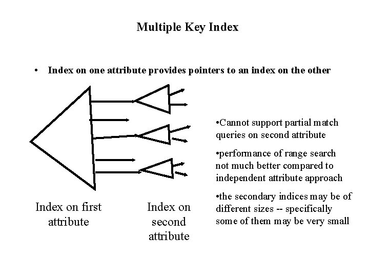
Multiple Key Index • Index on one attribute provides pointers to an index on the other • Cannot support partial match queries on second attribute • performance of range search not much better compared to independent attribute approach Index on first attribute Index on second attribute • the secondary indices may be of different sizes -- specifically some of them may be very small

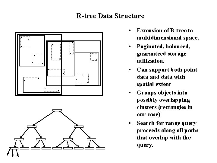
R-tree Data Structure • Extension of B-tree to multidimensional space. • Paginated, balanced, guaranteed storage utilization. • Can support both point data and data with spatial extent • Groups objects into possibly overlapping clusters (rectangles in our case) • Search for range query proceeds along all paths that overlap with the query.

R-tree Insert Object E • Step I 1 – Chooseleaf L to Insert E /* find position to insert*/ • Step I 2 – If L has room install E – Else Split. Node(L) • Step I 3: – Adjust Tree /* propagate Changes*/ • Step I 4: – if node split propagates to root adjust height of tree

Choose. Leaf • Step CL 1: – Set N to be root • Step CL 2: – If N is a leaf return N • Step CL 3: – If N is not a root, let F be an entry whose rectangle needs least enlargement to include object • break ties by choosing smaller rectangle • Step CL 4 – Set N to be child node pointed by entry F – goto Step CL 2

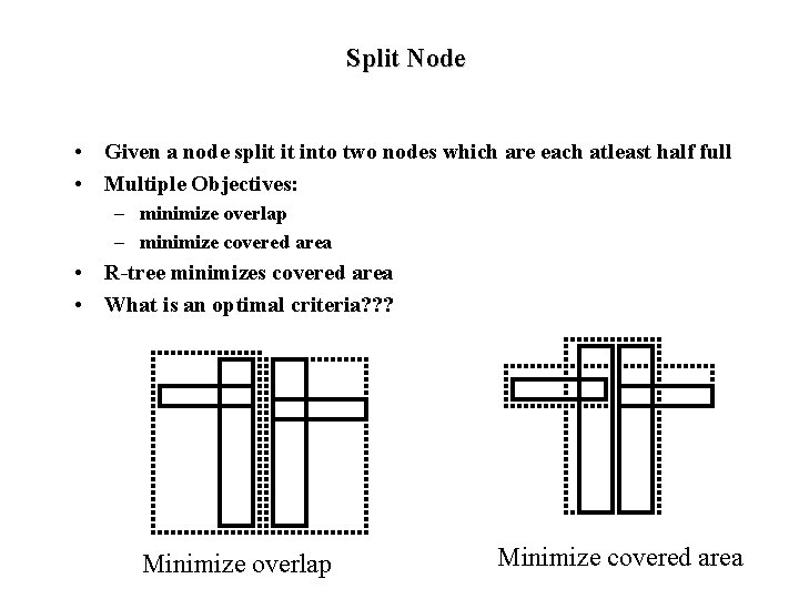
Split Node • Given a node split it into two nodes which are each atleast half full • Multiple Objectives: – minimize overlap – minimize covered area • R-tree minimizes covered area • What is an optimal criteria? ? ? Minimize overlap Minimize covered area

Minimizing Covered Area • • Group objects into 2 parts such that the covered area is minimized NP Hard!! Hence use heuritics Two heuristics explored – quadratic and linear

Basic Split Strategy • /* Divide the set of M+1 entries into 2 groups G 1 and G 2 */ • Pick. Seeds for G 1 and G 2 • Invoke Pick. Next to assign an object to a group recursively until either all objects assigned or one of the groups becomes half full. • If one group gets half full assign rest of the objects to the other group.

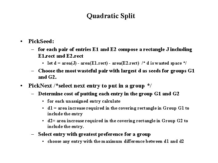
Quadratic Split • Pick. Seed: – for each pair of entries E 1 and E 2 compose a rectangle J including E 1. rect and E 2. rect • let d = area(J) - area(E 1. rect) - area(E 2. rect) /* d is wasted space */ – Choose the most wasteful pair with largest d as seeds for groups G 1 and G 2. • Pick. Next /*select next entry to put in a group */ – Determine cost of putting each entry in the group G 1 and G 2 • for each unassigned entry calculate • d 1 = area increase required in the covering rectangle in Group G 1 to include the entry • d 2= area increase required in the covering rectangle in Group G 2 to include the entry. – Select entry with greatest preference for a group • choose any entry with the maximum difference between d 1 and d 2

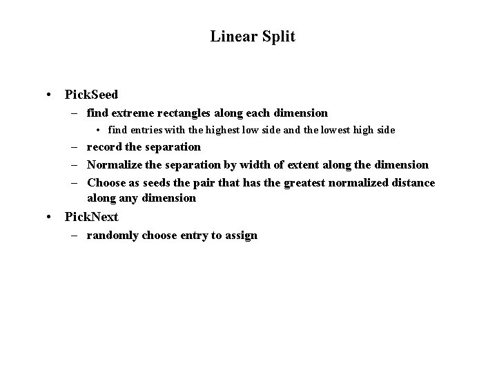
Linear Split • Pick. Seed – find extreme rectangles along each dimension • find entries with the highest low side and the lowest high side – record the separation – Normalize the separation by width of extent along the dimension – Choose as seeds the pair that has the greatest normalized distance along any dimension • Pick. Next – randomly choose entry to assign

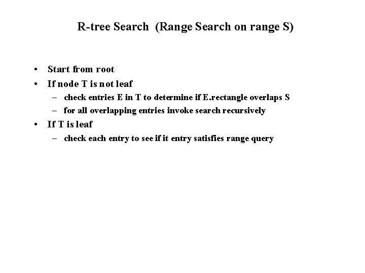
R-tree Search (Range Search on range S) • Start from root • If node T is not leaf – check entries E in T to determine if E. rectangle overlaps S – for all overlapping entries invoke search recursively • If T is leaf – check each entry to see if it entry satisfies range query

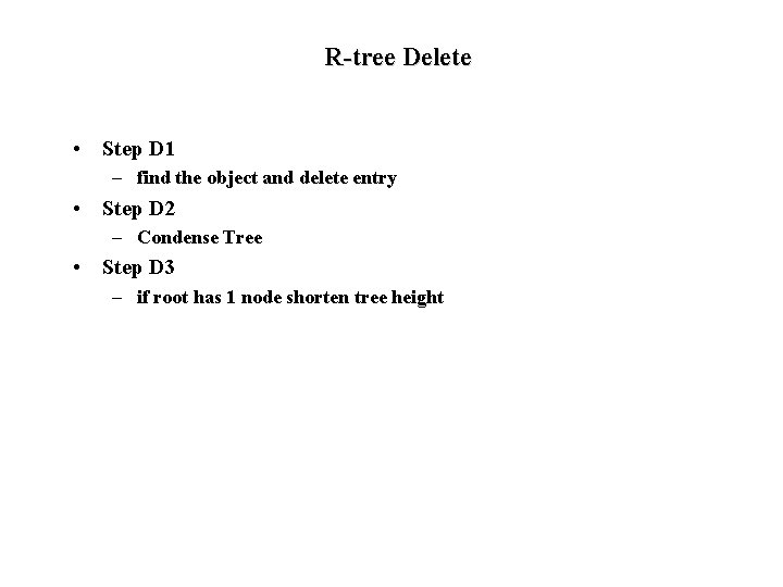
R-tree Delete • Step D 1 – find the object and delete entry • Step D 2 – Condense Tree • Step D 3 – if root has 1 node shorten tree height

Condense Tree • If node is underful – delete entry from parent and add to a set Q • Adjust bounding rectangle of parent • Do the above recursively for all levels • Reinsert all the orphaned entries – insert entries at the same level they were deleted.

Other Multidimensional Data Structures • Many generalizations of R-tree – different splitting criteria – different shapes of clusters (e. g. , d-dimensional spheres) – adding redundancy to reduce search cost: • store objects in multiple rectangles instead of a single rectangle to reduce cost of retrieval. But now insert has to store objects in many clusters. This strategy also increases overlap causing search performance to detoriate. • Space Partitioning Data Structures – unlike R-tree which group objects into possibly overlapping clusters, these methods attempt to partition space into non-overlapping regions. – E. g. , KD tree, quad tree, grid files, KD-Btree, HB-tree, hybrid tree. • Space filling curves – superimpose an ordering on multidimensional space that preserves proximity in multidimensional space. (Z-ordering, hilbert ordering) – Use a B-tree as an index on that ordering

KD-tree • A main memory data structure based on binary search trees – can be adapted to block model of storage (KD-Btree) • Levels rotate among the dimensions, partitioning the space based on a value for that dimension • KD-tree is not necessarily balanced.

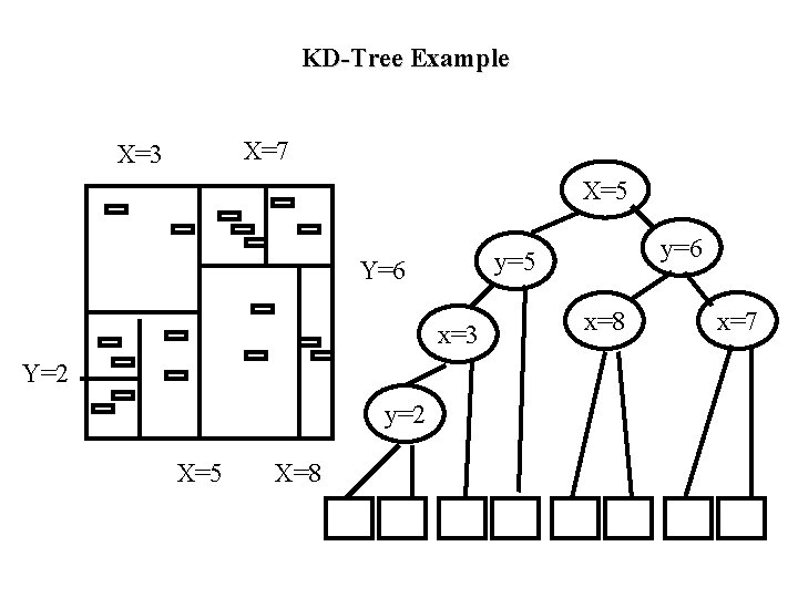
KD-Tree Example X=7 X=3 X=5 Y=6 x=3 Y=2 y=2 X=5 X=8 y=6 y=5 x=8 x=7

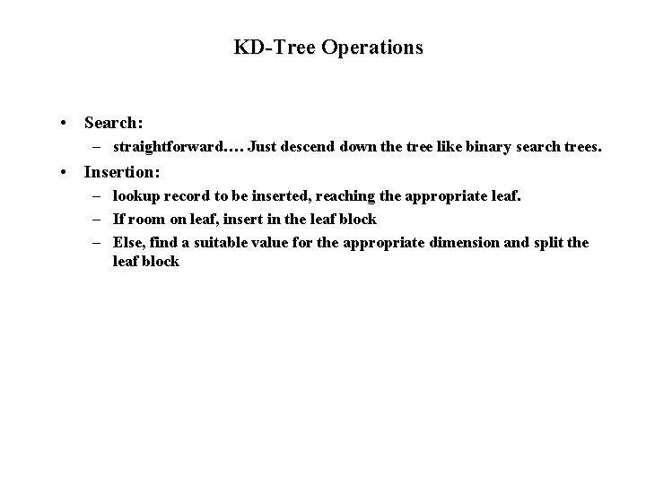
KD-Tree Operations • Search: – straightforward…. Just descend down the tree like binary search trees. • Insertion: – lookup record to be inserted, reaching the appropriate leaf. – If room on leaf, insert in the leaf block – Else, find a suitable value for the appropriate dimension and split the leaf block

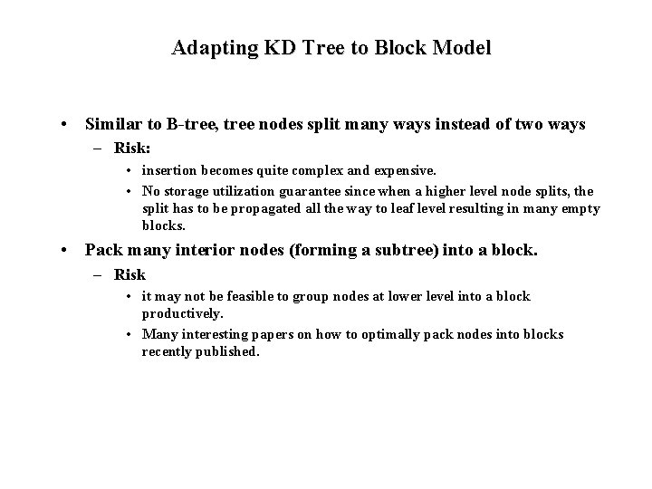
Adapting KD Tree to Block Model • Similar to B-tree, tree nodes split many ways instead of two ways – Risk: • insertion becomes quite complex and expensive. • No storage utilization guarantee since when a higher level node splits, the split has to be propagated all the way to leaf level resulting in many empty blocks. • Pack many interior nodes (forming a subtree) into a block. – Risk • it may not be feasible to group nodes at lower level into a block productively. • Many interesting papers on how to optimally pack nodes into blocks recently published.

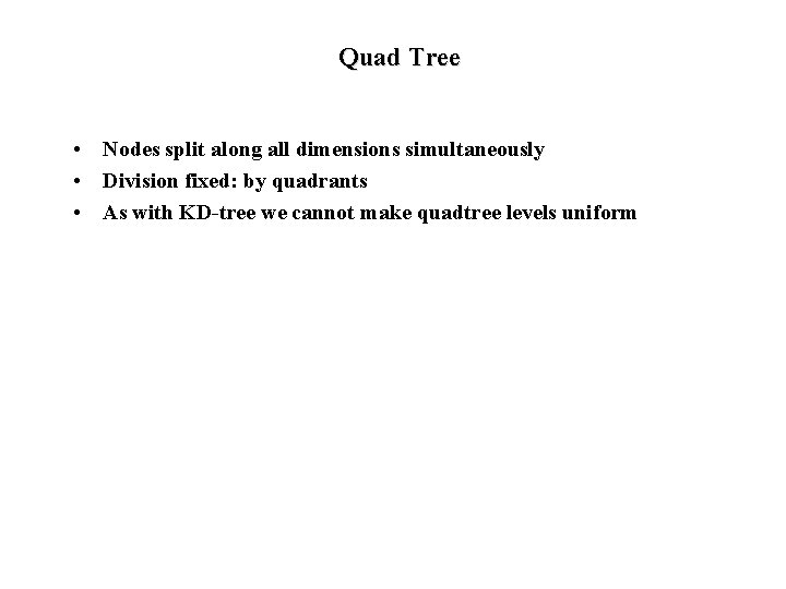
Quad Tree • Nodes split along all dimensions simultaneously • Division fixed: by quadrants • As with KD-tree we cannot make quadtree levels uniform

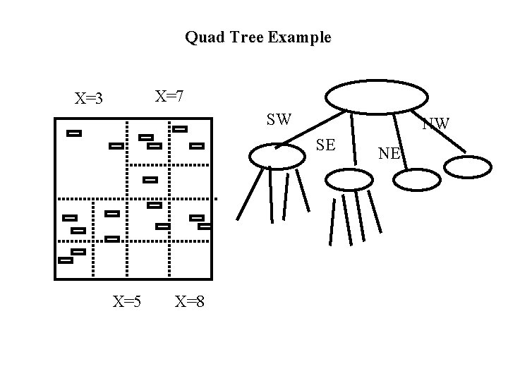
Quad Tree Example X=7 X=3 SW NW SE X=5 X=8 NE

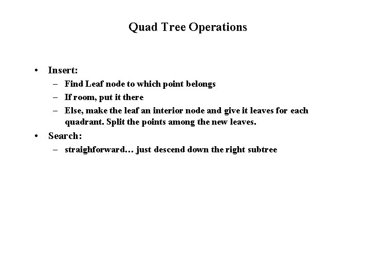
Quad Tree Operations • Insert: – Find Leaf node to which point belongs – If room, put it there – Else, make the leaf an interior node and give it leaves for each quadrant. Split the points among the new leaves. • Search: – straighforward… just descend down the right subtree

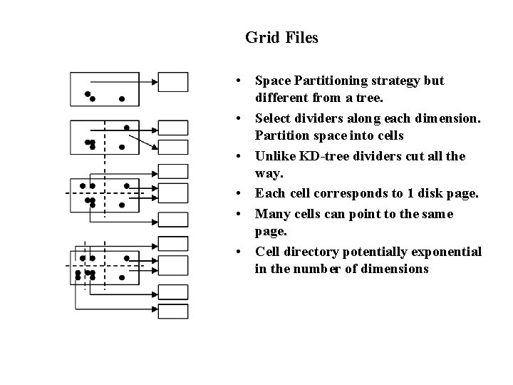
Grid Files • Space Partitioning strategy but different from a tree. • Select dividers along each dimension. Partition space into cells • Unlike KD-tree dividers cut all the way. • Each cell corresponds to 1 disk page. • Many cells can point to the same page. • Cell directory potentially exponential in the number of dimensions

Grid File Implementation • Maintain linear scales for each dimension that contain split positions for the dimension • Cell directory implemented as a multidimensional array. – /* can be large and may not fit in memory */

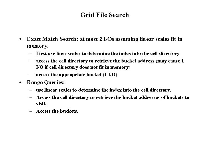
Grid File Search • Exact Match Search: at most 2 I/Os assuming linear scales fit in memory. – First use liner scales to determine the index into the cell directory – access the cell directory to retrieve the bucket address (may cause 1 I/O if cell directory does not fit in memory) – access the appropriate bucket (1 I/O) • Range Queries: – use linear scales to determine the index into the cell directory. – Access the cell directory to retrieve the bucket addresses of buckets to visit. – Access the buckets.

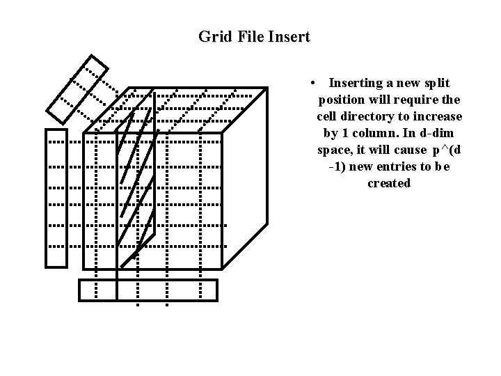
Grid File Insert • Determine the bucket into which insertion must occur. • If space in bucket, insert. • Else, split bucket – how to choose a good dimension to split? • If bucket split causes a cell directory to split do so and adjust linear scales. • /* notice that cell directory split results in p^(d-1) new entries to be created in cell directory */ • insertion of these new entries potentially requires a complete reorganization of the cell directory--- expensive!!!

Grid File Insert • Inserting a new split position will require the cell directory to increase by 1 column. In d-dim space, it will cause p^(d -1) new entries to be created

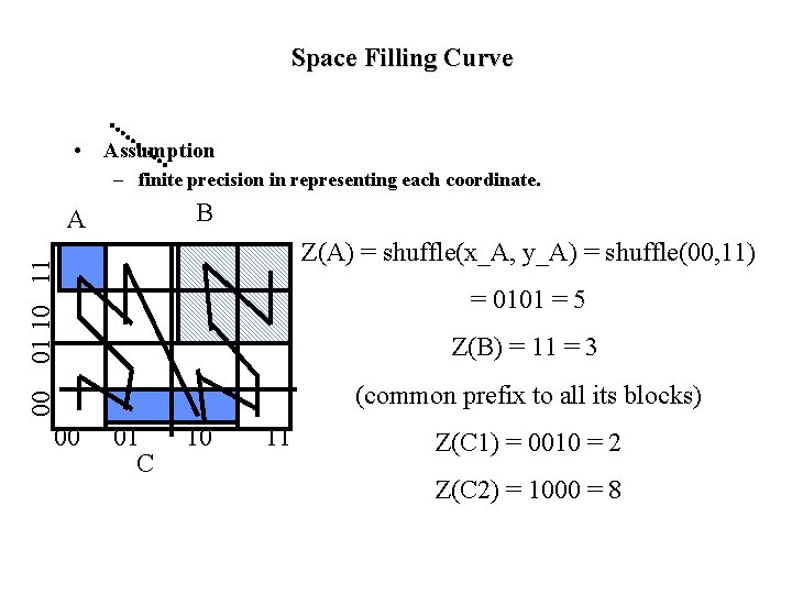
Space Filling Curve • Assumption – finite precision in representing each coordinate. B A 01 10 11 Z(A) = shuffle(x_A, y_A) = shuffle(00, 11) = 0101 = 5 Z(B) = 11 = 3 00 (common prefix to all its blocks) 00 01 C 10 11 Z(C 1) = 0010 = 2 Z(C 2) = 1000 = 8

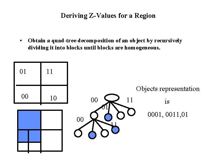
Deriving Z-Values for a Region • Obtain a quad-tree decomposition of an object by recursively dividing it into blocks until blocks are homogeneous. 01 00 11 Objects representation 10 00 00 11 01 is 0001, 0011, 01 11

Disk Based Storage • For disk storage, represent object based on its Z-value • Use a B-tree index. • Range Query: – translate query range to Z values – search B-tree with Z-values of data regions for matches

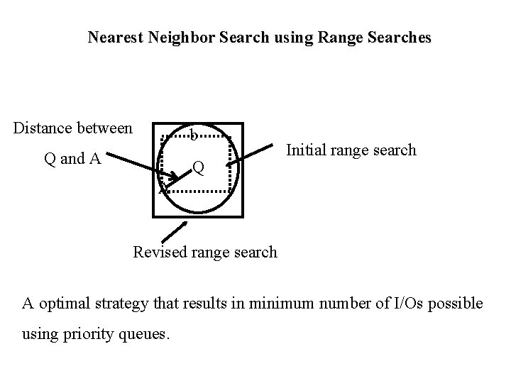
Nearest Neighbor Search • Retrieve the nearest neighbor of query point Q • Simple Strategy: – convert the nearest neighbor search to range search. – Guess a range around Q that contains at least one object say O • if the current guess does not include any answers, increase range size until an object found. – Compute distance d’ between Q and O – re-execute the range query with the distance d’ around Q. – Compute distance of Q from each retrieved object. The object at minimum distance is the nearest neighbor!!! Why? – Issues: how to guess range, the retrieval may be sub-optimal if incorrect range guessed. Becomes a problem in high dimensional spaces.

Nearest Neighbor Search using Range Searches Distance between b Q and A Q Initial range search A Revised range search A optimal strategy that results in minimum number of I/Os possible using priority queues.

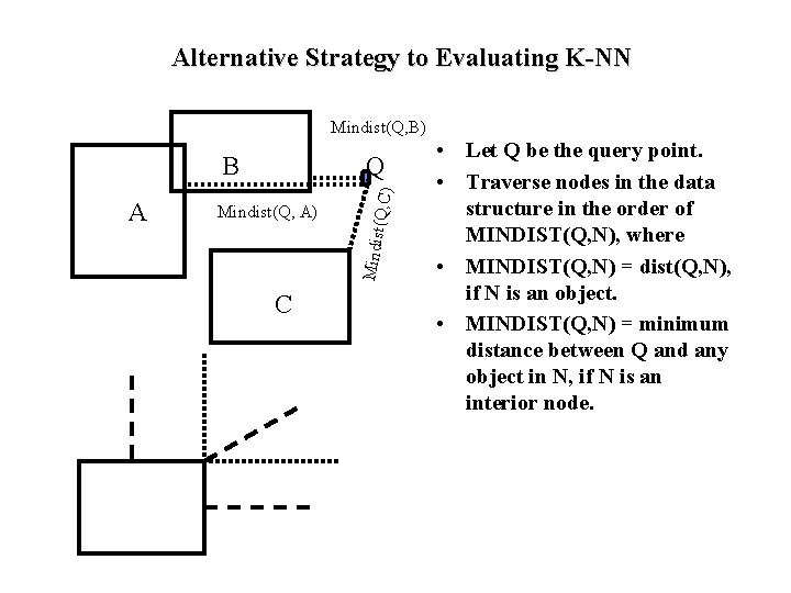
Alternative Strategy to Evaluating K-NN Mindist(Q, B) Mindist(Q, A) Mindist A Q (Q, C) B C • Let Q be the query point. • Traverse nodes in the data structure in the order of MINDIST(Q, N), where • MINDIST(Q, N) = dist(Q, N), if N is an object. • MINDIST(Q, N) = minimum distance between Q and any object in N, if N is an interior node.

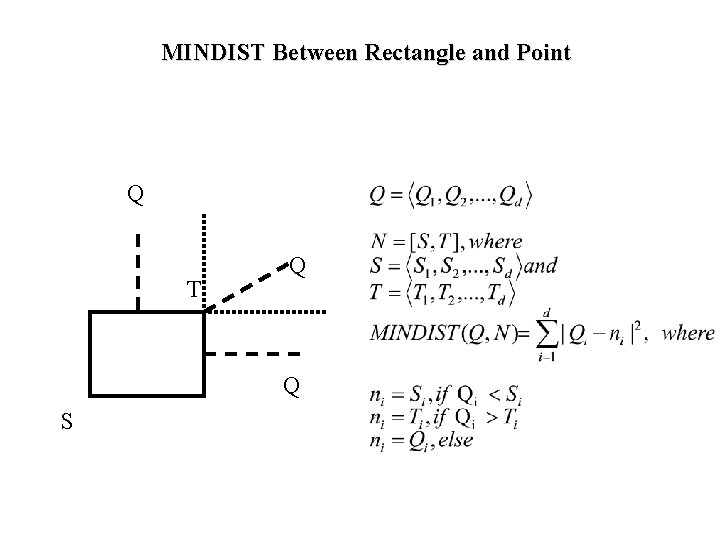
MINDIST Between Rectangle and Point Q T Q Q S

Generalized Search Trees • Motivation: – disparate applications require different data structures and access methods. – Requires separate code for each data structure to be integrated with the database code • too much effort. • Vendors will not spend time and energy unless application very important or data structure has general applicability. • Generalized search trees abstract the notion of data structure into a template. – Basic observation: most data structures are similar and a lot of book keeping and implementation details are the same. – Different data structures can be seen as refinements of basic Gi. ST structure. Refinements specified by providing a registering a bunch of functions per data structure to the Gi. ST.

Gi. ST supports extensibility both in terms of data types and queries • • • Gi. ST is like a “template” - it defines its interface in terms of ADT rather than physical elements (like nodes, pointers etc. ) The access method (AM) can customize Gi. ST by defining his or her own ADT class i. e. you just define the ADT class, you have your access method implemented! No concern about search/insertion/deletion, structural modifications like node splits etc.

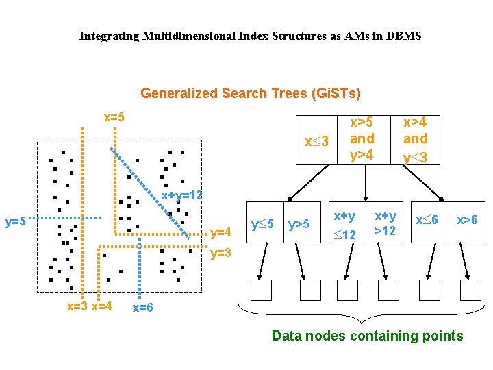
Integrating Multidimensional Index Structures as AMs in DBMS Generalized Search Trees (Gi. STs) x=5 x£ 3 x>5 and y>4 x>4 and y£ 3 x+y=12 y=5 y=4 y£ 5 y>5 x+y £ 12 x+y >12 x£ 6 x>6 y=3 x=4 x=6 Data nodes containing points

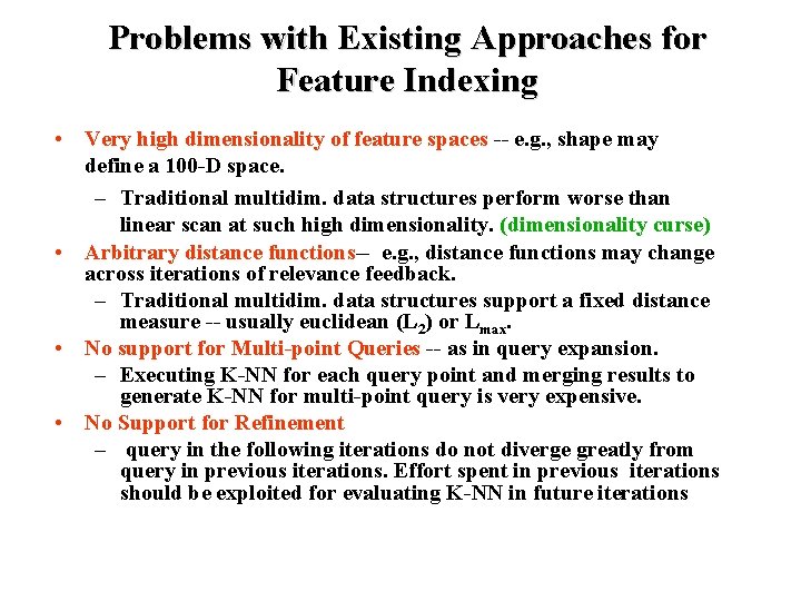
Problems with Existing Approaches for Feature Indexing • Very high dimensionality of feature spaces -- e. g. , shape may define a 100 -D space. – Traditional multidim. data structures perform worse than linear scan at such high dimensionality. (dimensionality curse) • Arbitrary distance functions-- e. g. , distance functions may change across iterations of relevance feedback. – Traditional multidim. data structures support a fixed distance measure -- usually euclidean (L 2) or Lmax. • No support for Multi-point Queries -- as in query expansion. – Executing K-NN for each query point and merging results to generate K-NN for multi-point query is very expensive. • No Support for Refinement – query in the following iterations do not diverge greatly from query in previous iterations. Effort spent in previous iterations should be exploited for evaluating K-NN in future iterations

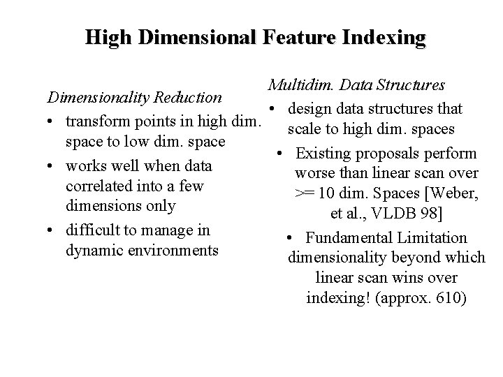
High Dimensional Feature Indexing Multidim. Data Structures Dimensionality Reduction • design data structures that • transform points in high dim. scale to high dim. spaces space to low dim. space • Existing proposals perform • works well when data worse than linear scan over correlated into a few >= 10 dim. Spaces [Weber, dimensions only et al. , VLDB 98] • difficult to manage in • Fundamental Limitation dynamic environments dimensionality beyond which linear scan wins over indexing! (approx. 610)

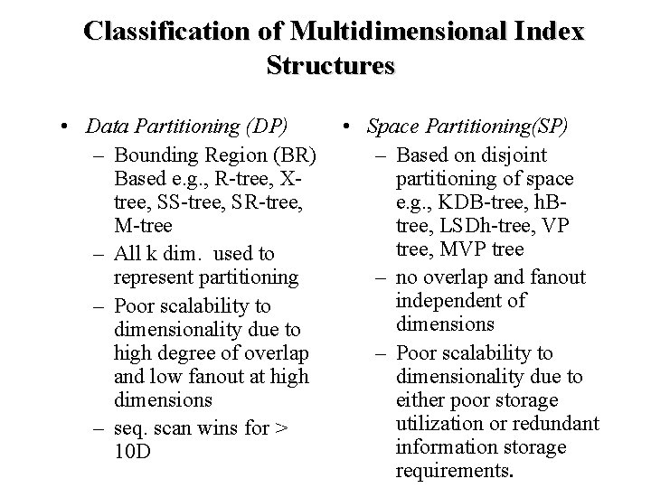
Classification of Multidimensional Index Structures • Data Partitioning (DP) – Bounding Region (BR) Based e. g. , R-tree, Xtree, SS-tree, SR-tree, M-tree – All k dim. used to represent partitioning – Poor scalability to dimensionality due to high degree of overlap and low fanout at high dimensions – seq. scan wins for > 10 D • Space Partitioning(SP) – Based on disjoint partitioning of space e. g. , KDB-tree, h. Btree, LSDh-tree, VP tree, MVP tree – no overlap and fanout independent of dimensions – Poor scalability to dimensionality due to either poor storage utilization or redundant information storage requirements.

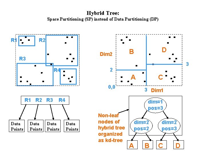
Hybrid Tree: Space Partitioning (SP) instead of Data Partitioning (DP) R 1 R 2 Dim 2 R 3 D B 3 2 R 4 A 0, 0 R 1 R 2 R 3 Data Points 3 Dim 1 R 4 Data Points C dim=1 pos=3 Data Points Non-leaf nodes of hybrid tree organized as kd-tree dim=2 pos=2 A B dim=2 pos=3 C D

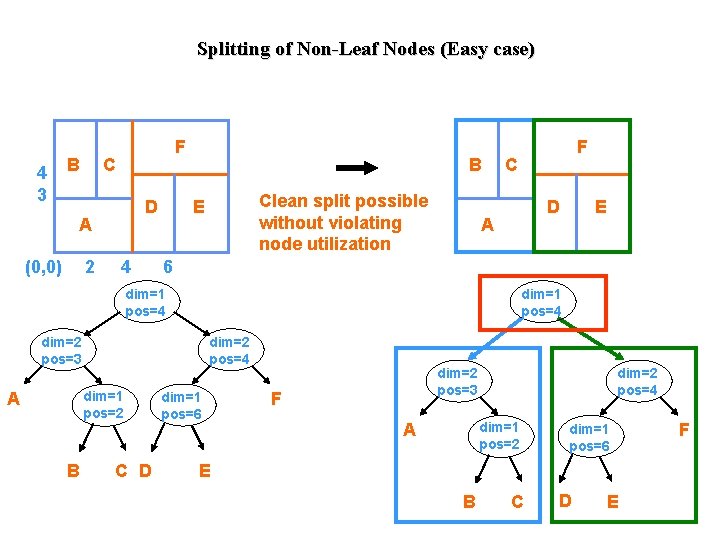
Splitting of Non-Leaf Nodes (Easy case) 4 3 B F C D A (0, 0) 2 4 B Clean split possible without violating node utilization E C D A dim=1 pos=4 dim=2 pos=3 dim=2 pos=4 dim=1 pos=2 B C D E 6 dim=1 pos=4 A F dim=1 pos=6 dim=2 pos=3 F dim=2 pos=4 dim=1 pos=2 A dim=1 pos=6 E B C D E F

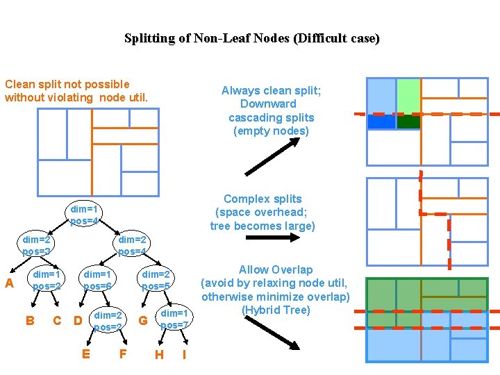
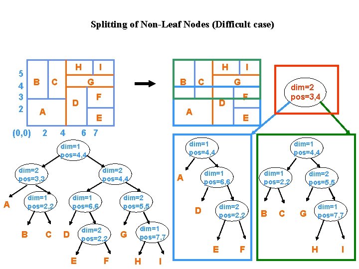
Splitting of Non-Leaf Nodes (Difficult case) Clean split not possible without violating node util. Always clean split; Downward cascading splits (empty nodes) Complex splits (space overhead; tree becomes large) dim=1 pos=4 dim=2 pos=3 A dim=2 pos=4 dim=1 pos=2 B dim=1 pos=6 C D E dim=2 pos=5 dim=2 pos=2 F G dim=1 pos=7 H I Allow Overlap (avoid by relaxing node util, otherwise minimize overlap) (Hybrid Tree)

Splitting of Non-Leaf Nodes (Difficult case) H 5 4 3 2 B C 2 H G B dim=2 pos=3, 3 A B F E dim=1 pos=4, 4 dim=2 pos=4, 4 C D dim=2 pos=3, 4 6 7 dim=1 pos=4, 4 dim=1 pos=2, 2 I G A E 4 C F D A (0, 0) I dim=1 pos=6, 6 dim=2 pos=2, 2 D G dim=1 pos=6, 6 A dim=2 pos=5, 5 F dim=1 pos=2, 2 dim=2 pos=2, 2 D B C dim=2 pos=5, 5 G dim=1 pos=7, 7 E E dim=1 pos=4, 4 H I F H I

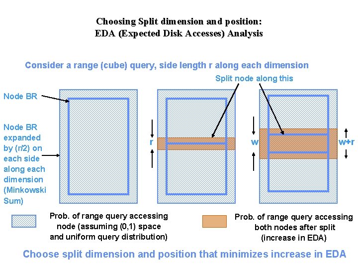
Choosing Split dimension and position: EDA (Expected Disk Accesses) Analysis Consider a range (cube) query, side length r along each dimension Split node along this Node BR expanded by (r/2) on each side along each dimension (Minkowski Sum) r Prob. of range query accessing node (assuming (0, 1) space and uniform query distribution) w w+r Prob. of range query accessing both nodes after split (increase in EDA) Choose split dimension and position that minimizes increase in EDA

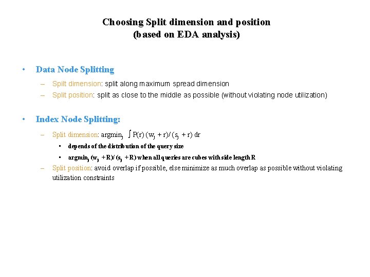
Choosing Split dimension and position (based on EDA analysis) • Data Node Splitting – Spilt dimension: split along maximum spread dimension – Split position: split as close to the middle as possible (without violating node utilization) • Index Node Splitting: – – Split dimension: argminj ò P(r) (wj + r)/ (sj + r) dr • depends of the distribution of the query size • argminj (wj + R)/ (sj + R) when all queries are cubes with side length R Split position: avoid overlap if possible, else minimize as much overlap as possible without violating utilization constraints

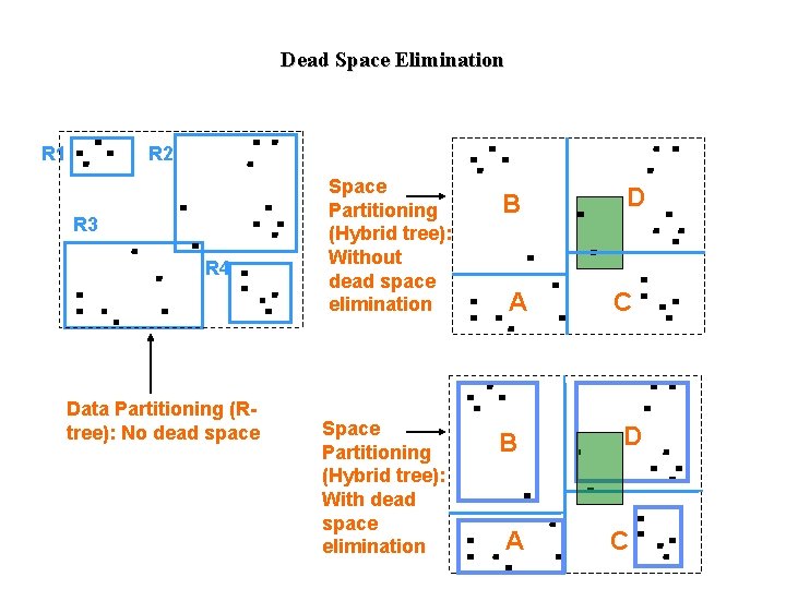
Dead Space Elimination R 1 R 2 R 3 R 4 Data Partitioning (Rtree): No dead space Space Partitioning (Hybrid tree): Without dead space elimination Space Partitioning (Hybrid tree): With dead space elimination B A D C

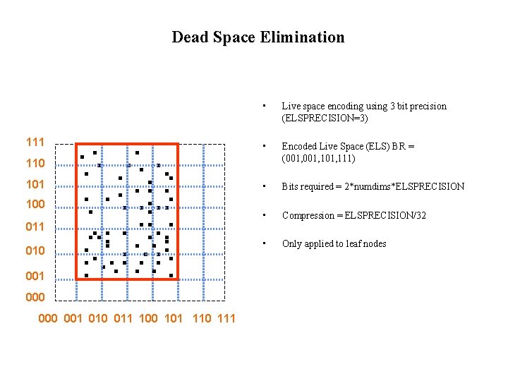
Dead Space Elimination 111 • Live space encoding using 3 bit precision (ELSPRECISION=3) • Encoded Live Space (ELS) BR = (001, 101, 111) • Bits required = 2*numdims*ELSPRECISION • Compression = ELSPRECISION/32 • Only applied to leaf nodes 110 101 100 011 010 001 000 001 010 011 100 101 110 111

Tree operations • • • Search: – Point, Range, NN-search, distance-based search as in DP-techniques – Reason: BR representation can be derived from kd-tree representation – Exploit tree organization (pruning) for fast intra-node search Insertion: – recursively choose space partition that contains the point – break tries arbitrarily – no volume computation (otherwise floating point exception at high dims) Deletion: – details in thesis

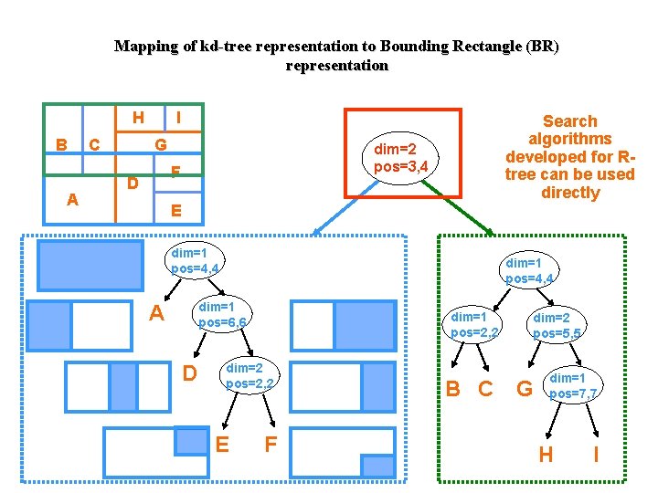
Mapping of kd-tree representation to Bounding Rectangle (BR) representation H B A C I G dim=2 pos=3, 4 F D Search algorithms developed for Rtree can be used directly E dim=1 pos=4, 4 dim=1 pos=6, 6 A D dim=1 pos=2, 2 dim=2 pos=2, 2 E F B C dim=2 pos=5, 5 G dim=1 pos=7, 7 H I

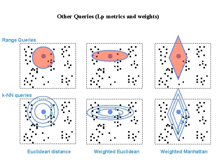
Other Queries (Lp metrics and weights) Range Queries k-NN queries 1 2 3 2 1 3 2 Euclidean distance Weighted Euclidean Weighted Manhattan

Advantages of Hybrid Tree • More scalable to high dimensionalities than: – DP techniques (R-tree like index structures) • Fanout independent of dimensionality: high fanout even at high dims • Faster intranode search due to kd-tree-based organization • No overlap at lowest level, low overlap at higher levels – SP techniques • Guaranteed node utilization • No costly cascading splits • EDA-optimal choice of splits • Supports arbitrary distance functions

Experiments • Effect of ELS encoding • Test scalability of hybrid tree to high dimensionalities – Compare performance of hybrid tree with SR-tree (data partitioning), h. B-tree (space partitioning) and sequential scan • Data Sets – Fourier Data set (16 -d Fourier vectors, 1. 2 million) – Color Histograms for COREL images (64 -d color histograms from 70 K images)

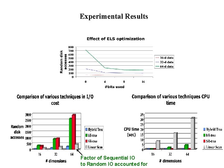
Experimental Results Factor of Sequential IO to Random IO accounted for

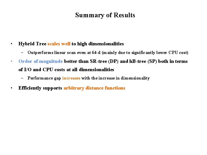
Summary of Results • Hybrid Tree scales well to high dimensionalities – Outperforms linear scan even at 64 -d (mainly due to significantly lower CPU cost) • Order of magnitude better than SR-tree (DP) and h. B-tree (SP) both in terms of I/O and CPU costs at all dimensionalities – Performance gap increases with the increase in dimensionality • Efficiently supports arbitrary distance functions

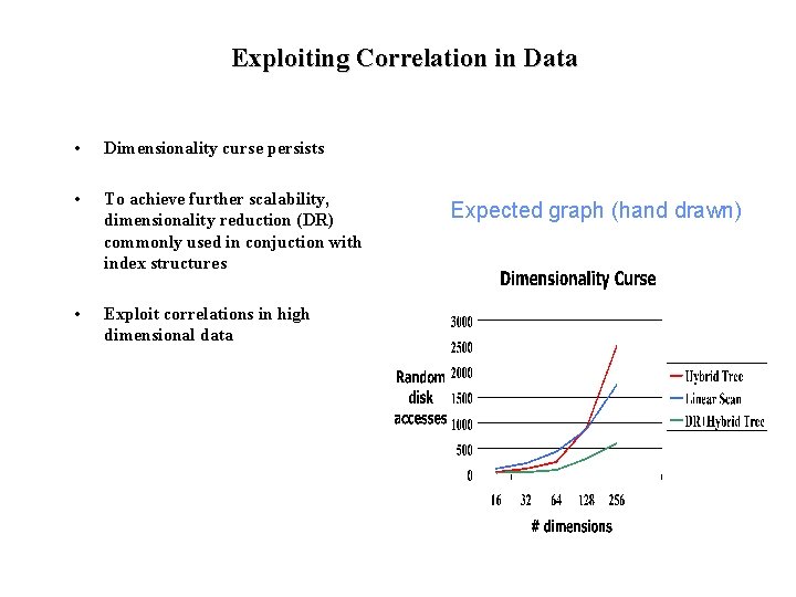
Exploiting Correlation in Data • Dimensionality curse persists • To achieve further scalability, dimensionality reduction (DR) commonly used in conjuction with index structures • Exploit correlations in high dimensional data Expected graph (hand drawn)

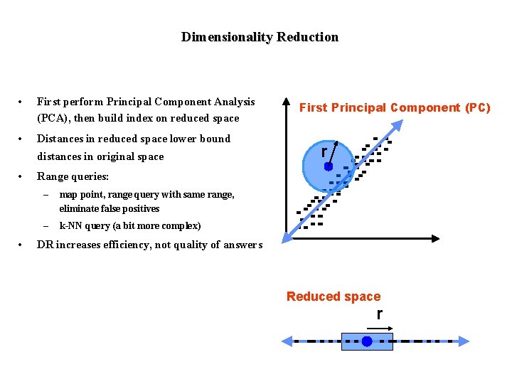
Dimensionality Reduction • First perform Principal Component Analysis (PCA), then build index on reduced space • Distances in reduced space lower bound distances in original space • • First Principal Component (PC) r Range queries: – map point, range query with same range, eliminate false positives – k-NN query (a bit more complex) DR increases efficiency, not quality of answers Reduced space r

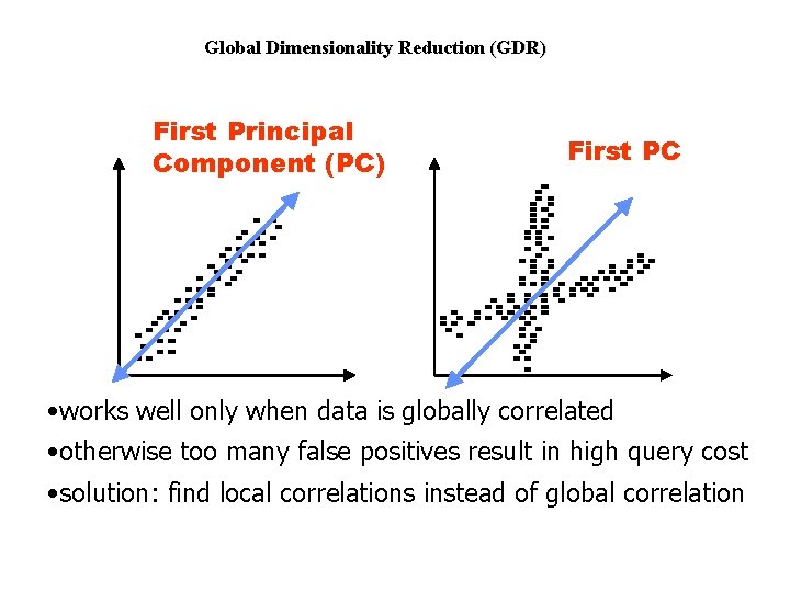
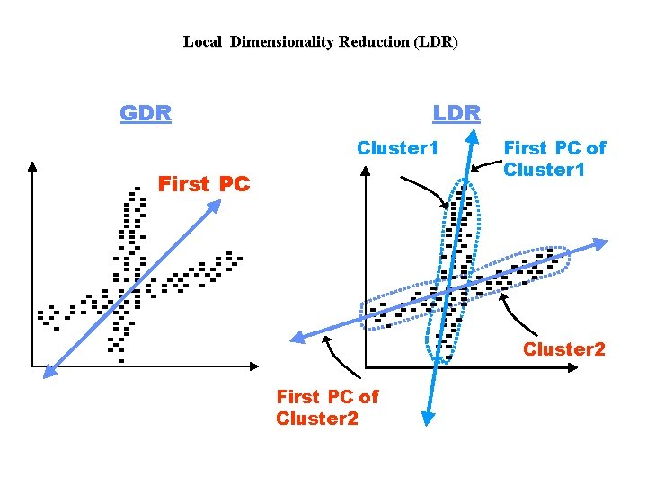
Global Dimensionality Reduction (GDR) First Principal Component (PC) First PC • works well only when data is globally correlated • otherwise too many false positives result in high query cost • solution: find local correlations instead of global correlation

Local Dimensionality Reduction (LDR) GDR LDR Cluster 1 First PC of Cluster 1 Cluster 2 First PC of Cluster 2

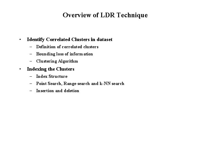
Overview of LDR Technique • Identify Correlated Clusters in dataset – Definition of correlated clusters – Bounding loss of information – Clustering Algorithm • Indexing the Clusters – Index Structure – Point Search, Range search and k-NN search – Insertion and deletion

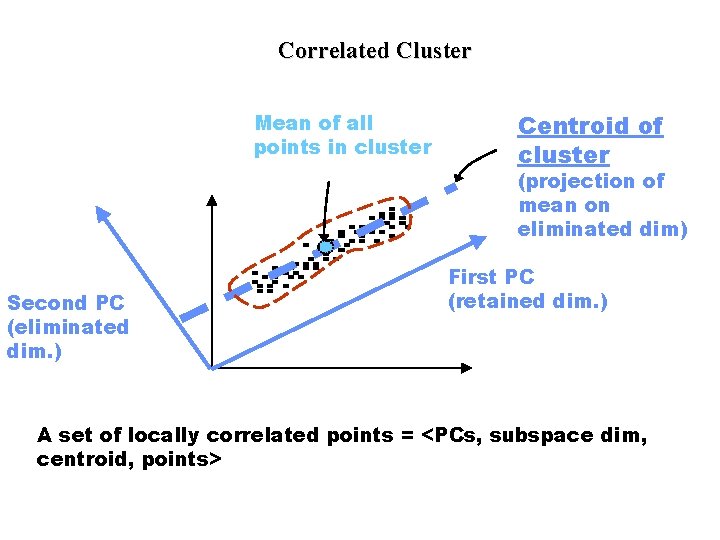
Correlated Cluster Mean of all points in cluster Centroid of cluster (projection of mean on eliminated dim) Second PC (eliminated dim. ) First PC (retained dim. ) A set of locally correlated points = <PCs, subspace dim, centroid, points>

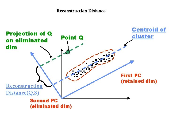
Reconstruction Distance Projection of Q on eliminated dim Point Q Reconstruction Distance(Q, S) Second PC (eliminated dim) Centroid of cluster First PC (retained dim)

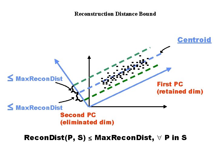
Reconstruction Distance Bound Centroid £ Max. Recon. Dist First PC (retained dim) £ Max. Recon. Dist Second PC (eliminated dim) Recon. Dist(P, S) £ Max. Recon. Dist, " P in S

Other constraints • Dimensionality bound: A cluster must not retain any more dimensions necessary and subspace dimensionality £ Max. Dim • Size bound: number of points in the cluster ³ Min. Size

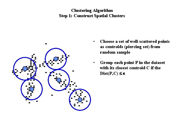
Clustering Algorithm Step 1: Construct Spatial Clusters • Choose a set of well-scattered points as centroids (piercing set) from random sample • Group each point P in the dataset with its closest centroid C if the Dist(P, C) £ e

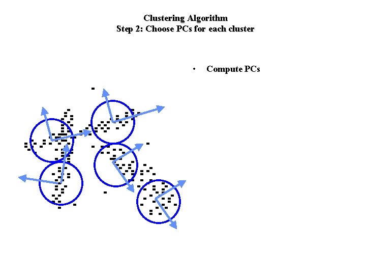
Clustering Algorithm Step 2: Choose PCs for each cluster • Compute PCs

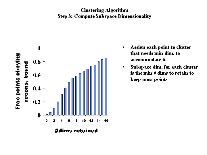
Clustering Algorithm Step 3: Compute Subspace Dimensionality • • Assign each point to cluster that needs min dim. to accommodate it Subspace dim. for each cluster is the min # dims to retain to keep most points

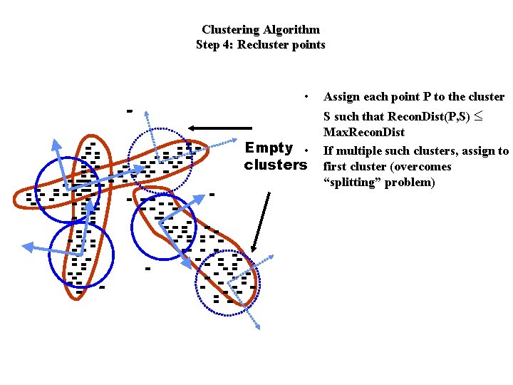
Clustering Algorithm Step 4: Recluster points • Empty • clusters Assign each point P to the cluster S such that Recon. Dist(P, S) £ Max. Recon. Dist If multiple such clusters, assign to first cluster (overcomes “splitting” problem)

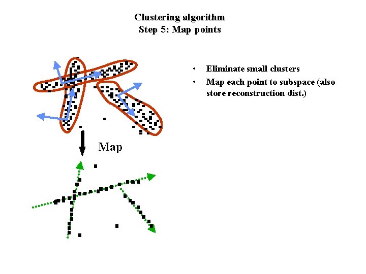
Clustering algorithm Step 5: Map points • • Map Eliminate small clusters Map each point to subspace (also store reconstruction dist. )

Clustering algorithm Step 6: Iterate • Iterate for more clusters as long as new clusters are being found among outliers • Overall Complexity: 3 passes, O(ND 2 K)

Experiments (Part 1) • Precision Experiments: – Compare information loss in GDR and LDR for same reduced dimensionality – Precision = |Orig. Space Result|/|Reduced Space Result| (for range queries) – Note: precision measures efficiency, not answer quality

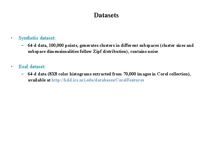
Datasets • Synthetic dataset: – 64 -d data, 100, 000 points, generates clusters in different subspaces (cluster sizes and subspace dimensionalities follow Zipf distribution), contains noise • Real dataset: – 64 -d data (8 X 8 color histograms extracted from 70, 000 images in Corel collection), available at http: //kdd. ics. uci. edu/databases/Corel. Features

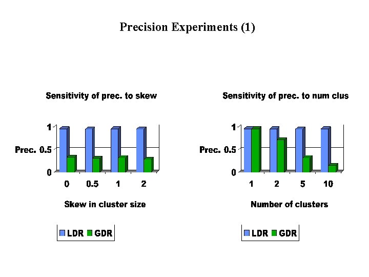
Precision Experiments (1)

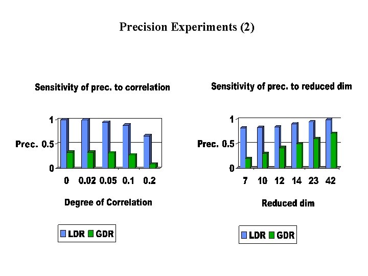
Precision Experiments (2)

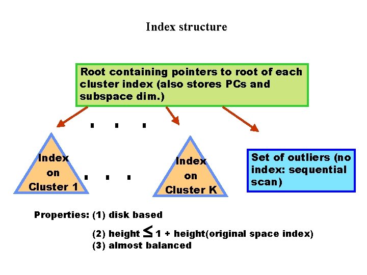
Index structure Root containing pointers to root of each cluster index (also stores PCs and subspace dim. ) Index on Cluster 1 Index on Cluster K Set of outliers (no index: sequential scan) Properties: (1) disk based £ (2) height 1 + height(original space index) (3) almost balanced

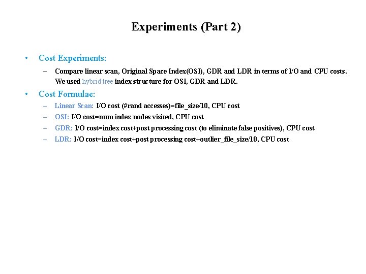
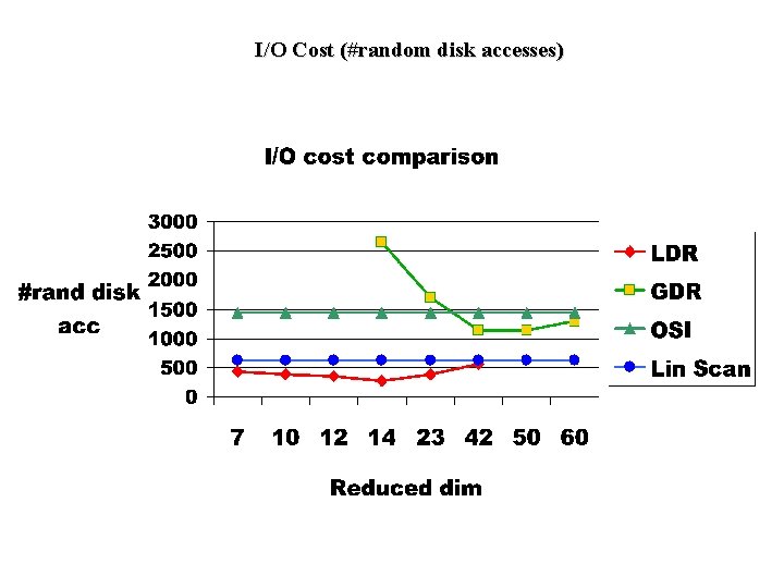
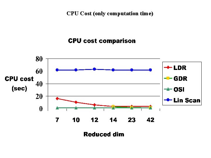
Experiments (Part 2) • Cost Experiments: – • Compare linear scan, Original Space Index(OSI), GDR and LDR in terms of I/O and CPU costs. We used hybrid tree index structure for OSI, GDR and LDR. Cost Formulae: – Linear Scan: I/O cost (#rand accesses)=file_size/10, CPU cost – OSI: I/O cost=num index nodes visited, CPU cost – GDR: I/O cost=index cost+post processing cost (to eliminate false positives), CPU cost – LDR: I/O cost=index cost+post processing cost+outlier_file_size/10, CPU cost

I/O Cost (#random disk accesses)

CPU Cost (only computation time)

Summary of LDR • • LDR is a powerful dimensionality reduction technique for high dimensional data – reduces dimensionality with lower loss in distance information compared to GDR – achieves significantly lower query cost compared to linear scan, original space index and GDR LDR is a general technique to deal with high dimensionality – our experience shows high dimensional datasets often have local correlations - LDR is the only technique that can discover/exploit it – applications beyond indexing: selectivity estimation, data mining etc. on high dimensional data (currently exploring)