Indexing and Retrieval Ales Franek Chunhui Zhu Gustave

Indexing and Retrieval Ales Franek Chunhui Zhu Gustave Granroth

Overview The goal is to design a system that can do accurate and efficient retrieval in a large image database(e. g. retrieval in movies. ). The first paper (video google) provides a fundamental framework to achieve this goal, other papers did some further improvement over the system.

CS 766 Paper Presentation Outline //Reference slide for presentation creation. Presentation Outline: 1. Introduction, some (but not all of the applications) of object/image searching. 2. High-level overview of the papers and their relation; also the relation of these papers with the presentations from the previous two groups. This includes a review of SIFT features. 3. Video Google (First Paper) a. Introduction; pipeline of the method. b. SA and MS regions of the image (feature finding) c. Feature clustering (via k-means). Association of features with words. -For videos: removing unstable regions (can be done efficiently). d. Dictionary building: describing image w/words -TF-IDF -Stop Lists e. Using spatial consistency to improve results and help with the ranking order. -15 point method (fast, but not as accurate) f. Retrieval - tree with inverted file. g. Performance, advantages, and disadvantages of this method. 4. Scalable Vocabulary Tree (Second Paper) a. Mention disadvantages of the first method (mainly speed and a small size). -First method also needs stop lists for good retrieval and takes longer on retrieval. b. Mention the general idea of this method. c. Scoring of the results, with the inverted files and virtual inverted files. d. Results, advantages, disadvantages. 5. City Scale Location Recognition (Third Paper) a. Mention the general idea of this method -- note it is an extension of (3, 4). b. Note the greedy algorithm used to run this method. c. Note the idea of information gain used to only use the nodes in the vocabulary tree that provide the most information. d. Results, Final conclusions of everything.

2. Video Google: A Text Retrieval Approach to Object Matching in Videos Josef Sivic and Andrew Zisserman, ICCV 2003. Goal: To retrieve key frames and shots of a video containing a particular object.

Much previous work has been done in the text retrieval area, the goal of this work is to borrow some successful ideas from text retrieval to make the visual object/frame retrieval from video faster and more accurate.

Text Retrieval Offline: Document contains words. Words parsed into their stems. e. g. 'walk', 'walking' and 'walks' will all be represented by the stem 'walk'. Stop list to reject common words such as 'the', 'a', 'is', etc. Each document is represented by a vector with components given by the frequency of the occurrence of the words the document contain. Online: Query is also parsed to words, then stems, and form a vector. Similarity of a document and a query is computed by computing vector similarity. • • •

Analog • • • Corpus ---- Film Document ---- Frame Stem ---- ? ? ? Word ---- ? ? ? Query ---- One frame or subpart of a frame

Textual Words -> Visual Words • • • Each frame(document) contain many local descriptors(words) A good descriptor should be invariant to different viewpoints, scales, illuminations, shifts and transformations. How to build? a. Find invariant regions in the frame b. Represent each detected invariant region by a descriptor

Finding Invariant Regions (1/2) • • Two types of 'viewpoint covariant regions' used: a. SA - Shape Adapted: tends to be centered on corner like features. b. MS - Maximally Stable: corresponds to blobs of high contrast with respect to their surroundings. Reason to use to two different region types: complementary representation of frames.

Finding Invariant Regions (2/2)

Building the Descriptors • • SIFT feature - Scale Invariant Feature Transform. Each elliptical region is represented by a 128 -dimensional vector. Removing noise: a. Tracking region using 'Constant Velocity Dynamical model', any region doesn't survive 3 frames is rejected. b. Regions throughout the track are averaged to improve SNR(Signal Noise Ratio). c. Regions with large covariance are also rejected.

Analog • • • Corpus ---- Film Document ---- Frame Stem ---- ? ? ? Word ---- Descriptor (Visual Word) Query ---- One frame or subpart of a frame

Building the 'Visual Stems' • • Cluster descriptors into K groups using K-means clustering. Each cluster represents a 'visual word' in the 'visual vocabulary'. For any arbitrary descriptor, find the nearest cluster center to it and assign with the visual word of that cluster. Analog to text stemming. 6 K SA clusters, and 10 K MS clusters.

Two Clusters of SA Regions Two Clusters of MS Regions

Analog • • • Corpus ---- Film Document ---- Frame Stem ---- Center of Descriptor Cluster Word ---- Descriptor (Visual Word) Query ---- One frame or subpart of a frame

Process Overview Offline: Vocabulary(Stem) building Crawl Frames Create Stop List Online: Build query vector Rank Result • • •

Vocabulary Building

Crawling Frames

Crawling Frames: tf-idf Each document is represented as a vector: k is the number of vocabulary, nid is the number of occurrence of word i in the document d, nd is the total number of words in document d, ni is the occurrence of word i in the whole database, and N is the number of documents in the whole database. The similarity of two documents(video frame or subpart of video frame here) is computed by the normalized dot product between their vectors

Crawling Frames: inverted index Given the texts T 1="it is what it is", T 2 ="what is it" and T 3="it is a banana", we have the following inverted file index: "a": {2} "banana": {2} "is": {0, 1, 2} "it": {0, 1, 2} "what": {0, 1} During query time, to find relevant frames quickly.

Query Object

Query Object: Ranking Result Ranking based on two parts: 1. 2. Vector similarity mentioned before: each frame is represented by a vector. . . Spatial Consistency

Two Experiments Scene Location Matching: Evaluate the method by matching scene locations across the movie. Used to tune the system. • • Object Retrieval

Scene Location Matching 164 frames, from 48 shots, were taken at 19 3 D location in the movie ‘Run Lola Run’ (4 -9 frames from each location)

Scene Location Matching

Object Retrieval • • • Search for objects of interest throughout the movie. The object of interests is specified by users as a sub part of any frame. http: //arthur. robots. ox. ac. uk: 8081/cgibin/shot_viewer/vg_single_image. py? frames+list=106725 &movie+name=charade

Video Google Summary • • • Provide a framework to do visual search in video Runtime object retrieval Open issues: a. Automatic way of building vocabulary, non-static vocabulary b. Undesirable low ranking caused by insufficient feature c. Scalability

3. Scalable Recognition with a Vocabulary Tree Nistér and Stewénius, CVPR 2006. Example image retrieval process given the query image of a shoe.

Vocabulary Tree (1: 2) -Hierarchy of k-means clusters, with a 'k' branch factor, of the local region descriptors. Illustration: Tree-building process, with k = 3. -Adding a new descriptor: 'k. L' dot products to determine the descriptor clusters. -Encoding descriptor location: Single integer with k/2 bits per level can encode the path. -Memory usage: D*k. L * (bits/descriptor) (143 MB with D=128, char=bits, k=10, L=6).

Vocabulary Tree (2: 2) Allows For: -Faster Retrieval. -Larger Vocabulary, Smaller Database Size. -Better Retrieval Quality. -No need for stop lists.

Scoring (1: 2) Video Google: Inverted files from a TF-IDF (term frequency-inverse document) scoring. Vocabulary Tree: Hierarchy of visual words in a vocabulary tree, with inverted files at the leaves. -Comparing similarity of paths in the vocabulary tree. Weight method (weights based on entropy): >> qi = niwi, di = miwi (Query and Database vectors) >> (Scoring) General Observations >> Weights should not be strong for inner nodes. >> Setting weights to 0 defines a stop list (optional). Illustration: 400 paths for the descriptors in a single image.

Scoring (2: 2) -Implemented with inverted files (id # of images with feature and feature frequency in each image) -Inverted file length ~ frequency. -Inner nodes consists of a concatenation of the leaf nodes inverted files. Illustration: Scoring with norms. Either L 1 or L 2 norms work well.

Results and Applications Result metrics: -- 0. 25 s for feature extraction on a 640 x 480 image; 5 Hz on-the-fly insertion to the database. -- 0. 025 (25 ms) query time with 50, 000 database images. -- Size of the database vs feasible verification. -- Real-time CD cover recognition. -- 1 s query time with 1, 000 database images (6 movies and 6, 376 image ground truth) -- 2. 5 days for database creation, mainly on feature extraction. -Fast object recognition. -General image query applications. Percentage of GT images making into the top x-percent frames from a 1, 400 image query.

4. City-Scale Location Recognition Schindler, Brown, and Szeliski, CVPR 2007. From left to right: Vehicle path during image database creation, a query image, and the match returned from the database.

Improvements to Vocabulary Trees - Improved feature matching via: - Improved vocabulary selection (faster retrieval, larger database size possible) - Generalized (and faster) search algorithm Differences in the Method - No hierarchical scoring - Focus on location, rather than object recognition.

Greedy N-Best Paths Search -Generalization to traditional vocabulary tree search method. -Instead of performing k. L comparisons at each level, k + k. N(L - 1) are performed (following N different paths). -Allows for a similar number of comparisons to be performed for different-branching trees.

Information Gain - Modeling the features that are most locationinformative, via high-gain training data.

Scoring -Scoring done via a voting scheme. -Matched features vote for the images they occur in. -Performance enhanced by normalizing by feature count in an image, number of nearest neighbors images, and local neighborhood images. -Vocabulary tree performs the sums in linear time.

Results (1: 2) - 10 million image dataset, analysis with 30, 000 image subset and 278 query images. Experiment 1: Informative Features -Constant 7. 5 million points, 3, 000 to 30, 000 images with gradual increase.

Results (2: 2) Experiment 2: Greedy N-Best Paths Algorithm -Apx 1, 000 features, variant tree branching factor. Also compared with a kd-tree.

Retrieving results

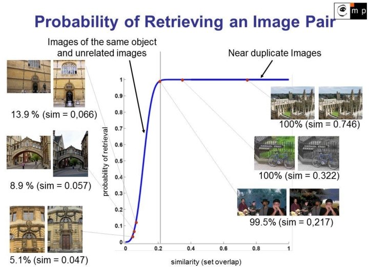
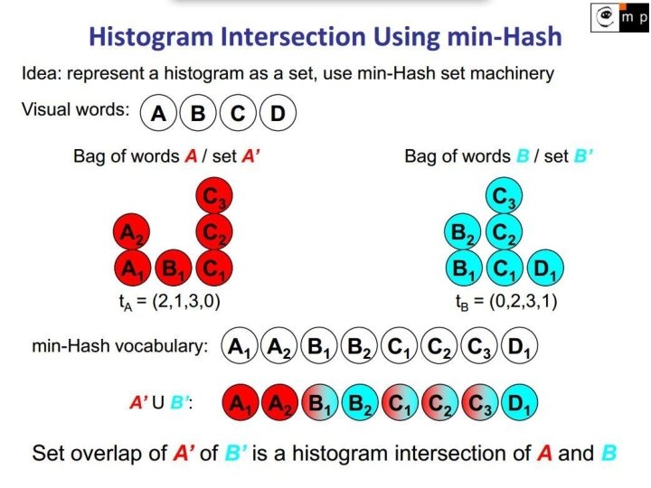
Min. Hash The min-wise independent permutations locality sensitive hashing scheme Quick estimation of similarity of two sets Proposed by Andrei Broder [On the resemblance and containment of documents, 1997] Used in Alta. Vista search engine to detect duplicate web pages and eliminate them from search results

Similarity measure Jaccard similarity coefficient J(A, B) = |A∩B| / |A∪B| Hash function h maps members of set S to distinct integers. hmin(S) is then the minimum hash value of all members of S. Pr[hmin(A) = hmin(B)] = J(A, B)

Key features Reducing estimating resemblance to set intersection problems Can be easily evaluated by a process of random sampling Bounded error expectation O(1/√k). For k = O(1/ε 2) samples is expected error at most ε Independently computed for each document (image) Fixed size sample for each document (image) Distance d(A, B) = 1 - J(A, B) is a metric (obeys the triangle inequality) Hash values can be weighted, e. g. tf-idf can be used

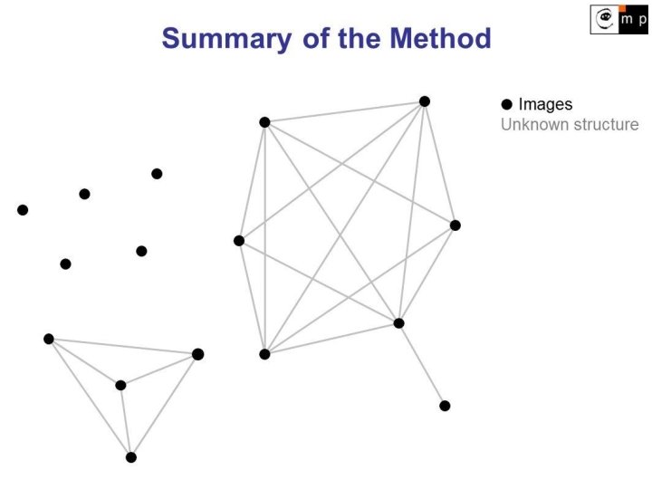
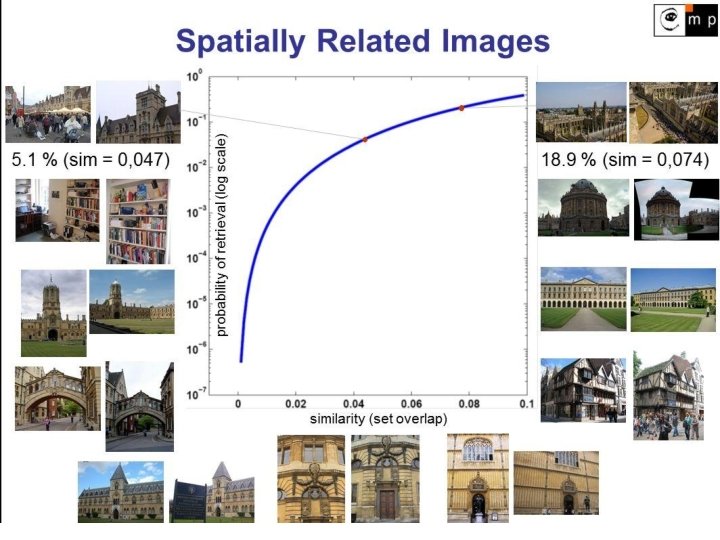
Large-Scale Discovery of Spatially Related Images [Chum, Matas 2010] Finding and matching all spatially related images in a large database Fast method, even for sizes up to 250 images Finding clusters of related images Visual only approach Probability of successful discovery independent of database size

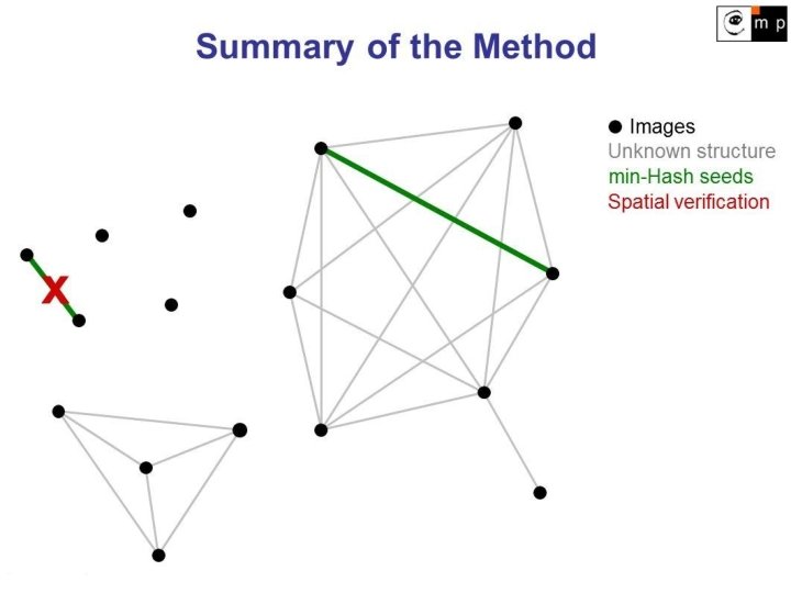
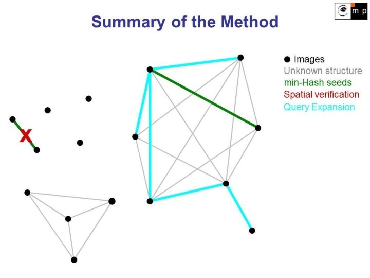
Key idea: 2 steps 1. Seed Generation (hashing) - fast, low recall Chum, Philbin, Isard, and Zisserman: Scalable Near Identical Image and Shot Detection, 2007 • used for detection of duplicate images 2. Seed Growing (retrieval) - high recall Chum, Philbin, Sivic, Isard, and Zisserman: Total Recall: Automatic Query Expansion with a Generative Feature Model for Object Retrieval, 2007 • used for expanding the query image description

1. Seed Generation: Probability of Success At least 1 out of k s-tuples of min-Hashes agrees: 1 - (1 - J(A, B)s)k where s is the size of the hashing table and k is number of hashing tables

Probability of finding seed P(no seed) = 68%

Probability of finding seed P(no seed) = 1. 94%

2. Seed Growing - Automatic Query Expansion

Query Expansion Example

Example of a Cluster

Conclusion Fast and accurate method useful for very large datasets Very low false positive rate Store small amount of data per image Easily parallelizable Much more new images can be retrieved thanks to query expansion Clusters are more efficient than just indexing

Thank you Ales Franek Chunhui Zhu Gustave Granroth