Indexes Primary Indexes Dense Indexes Pointer to every

Indexes

Primary Indexes Dense Indexes Pointer to every record of a sequential file, (ordered by search key). • Can make sense because records may be much bigger than key pointer pairs. - Fit index in memory, even if data file does not? - Faster search through index than data file? Sparse Indexes Key pointer pairs for only a subset of records, typically first in each block. • Saves index space.

Dense Index

Sparse Index

Num. Example of Dense Index • Data file = 1, 000 tuples that fit 10 at a time into a block of 4096 bytes (4 KB) • 100, 000 blocks data file = 400 MB • Index file: For typical values of key 30 Bytes, and pointer 8 Bytes, we can fit: 4096/(30+8) 100 (key, pointer) pairs in a block. • So, we need 10, 000 blocks = 40 MB for the index file. This might fit into the available main memory.

Num. Example of Sparse Index • Data file and block sizes as before • One (key, pointer) record for the first record of every block index file = 100, 000 (key, pointer) pairs = 100, 000 * 38 Bytes = 1, 000 blocks = 4 MB • If the index file could fit in main memory 1 disk I/O to find record given the key

Lookup for key K Sparse vs. dense? 1. Find key K in dense index. 2. Find largest key K in sparse index. Follow pointer. a) Dense: just follow. b) Sparse: follow to block, examine block. Dense vs. Sparse: Dense index can answer: ”Is there a record with key K? ” Sparse index can not!

Cost of Lookup • We can do binary search. • log 2 (number of index blocks) I/O’s to find the desired record. • All binary searches to the index will start at the block in the middle, then at 1/4 and 3/4 points, 1/8, 3/8, 5/8, 7/8. - So, if we store some of these blocks in main memory, I/O’s will be significantly lower. • For our example: Binary search in the index may use at most log 10, 000 = 14 blocks (or I/O’s) to find the record, given the key, … or much less if we store some of the index blocks as above.

Secondary Indexes • A primary index is an index on a sorted file. - Such an index “controls” the placement of records to be “primary, ” • A secondary index is an index that does not reflect data placement. - Sparse, secondary index makes no sense. - Usually, search key is not a “key. ”

Indirect Buckets • To avoid repeating keys in index, use a level of indirection, called buckets. • Additional advantage: allows intersection of sets of records without looking at records themselves.

Movies(title, year, length, studio. Name); SELECT title FROM Movies WHERE studio. Name = 'Disney' AND year = 1995; Secondary indexes on studio. Name and year.

Operations with Indexes • Deletions and insertions are problematic for flat indexes. • Eventually, we need to reorganize entries and records. - E. g. insert 15 …that’s a messy approach… Better: Use B Trees

B Trees: A typical leaf and interior node (unclusttered index) Leaf 81 57 95 To next leaf in sequence To record with key 57 Interior Node To subtree with keys K<57 To record with key 81 with key 95 57 81 To subtree with keys 57 K<81 57, 81, and 95 95 To subtree with keys 81 K<95 To subtree with keys K 95 are the least keys we can reach by via the corresponding pointers.

A typical leaf and interior node (clusttered index) Leaf 57 81 95 To next leaf in sequence Record with key 57 Interior Node To keys K<57 Record with key 81 with key 95 57 81 To keys 57 K<81 57, 81, and 95 95 To keys 81 K<95 To keys K 95 are the least keys we can reach by via the corresponding pointers.

Operations in B Tree • Will illustrate with unclustered case, but straightforward to generalize for the clustered case. Operations 1. Lookup 2. Insertion 3. Deletion

Lookup 13 7 2 3 5 7 23 11 13 17 19 31 23 Try to find a record with search key 40. 43 29 31 37 41 43 47 Recursive procedure: If we are at a leaf, look among the keys there. If the i th key is K, the i th pointer will take us to the desired record. If we are at an internal node with keys K 1, K 2, …, Kn, then if K<K 1 we follow the first pointer, if K 1 K<K 2 we follow the second pointer, and so on.

Try to insert a search key = 40. First, lookup for it, in order to find where to insert. Insertion 13 7 2 3 5 7 23 11 13 17 19 31 23 43 29 31 37 41 43 47 It has to go here, but the node is full!

Beginning of the insertion of key 40 13 7 2 3 5 7 23 11 13 17 19 31 23 43 29 31 What’s the problem? No parent yet for the new node! 43 37 40 Observe the new node and the redistribution of keys and pointers 41 47

Continuing of the Insertion of key 40 We must now insert a pointer to the new leaf into this node. We must also associate with this pointer the key 40, which is the least key reachable through the new leaf. But the node is full. Thus it too must split! 13 7 2 3 5 7 23 11 13 17 19 31 23 43 29 31 43 37 40 41 47

Completing of the Insertion of key 40 13 This is a new node. 7 2 3 5 7 23 11 13 17 19 43 31 23 • We have to redistribute 3 keys and 4 pointers. • We leave three pointers in the existing node and give two pointers to the new node. 43 goes to the new node. • But where the key 40 goes? • 40 is the least key reachable via the new node. 29 31 43 37 40 41 47

Completing of the Insertion of key 40 13 It goes here! 40 is the least key reachable via the new node. 40 7 2 3 5 7 23 11 13 17 19 43 31 23 29 31 43 37 40 41 47

Structure of B trees • Degree n means that all nodes have space for n search keys and n+1 pointers • Node = block • Let - block size be 4096 Bytes, - key 4 Bytes, - pointer 8 Bytes. • Let’s solve for n: 4 n + 8(n+1) 4096 n 340 n = degree = order = fanout

Example • n = 340, however a typical node has 255 keys • At level 3 we have: 2552 nodes, which means 2553 16 220 records can be indexed. • Suppose record = 1024 Bytes we can index a file of size 16 220 210 16 GB • If the root is kept in main memory accessing a record requires 3 disk I/O

Deletion Suppose we delete key=7 13 7 2 3 5 7 23 11 13 17 19 31 23 43 29 31 37 41 43 47

Deletion (Raising a key to parent) 13 5 23 11 13 17 19 This node is less than half full. So, it borrows key 5 from sibling. 31 23 43 29 31 37 41 43 47

Deletion Suppose we delete now key=11. No siblings with enough keys to borrow. 13 5 23 11 13 17 19 31 23 43 29 31 37 41 43 47

Deletion 13 23 2 3 5 13 17 19 31 23 43 29 We merge, i. e. delete a block from the index. However, the parent ends up not having any key. 31 37 41 43 47

Deletion 23 31 13 2 3 5 13 17 19 Parent: Borrow from sibling! 23 43 29 31 37 41 43 47

Inverted Indexes • Similar (to secondary indexes) idea from information retrieval community, but: - Record document. - Search keyvalue of record presence of a word in a document. • Usually used with “buckets. ”

Additional Information in Buckets • We can extend bucket to include role, position of word, e. g. Type Position

A Reuters RCV 1 document 1 GB collection of such documents

Reuters RCV 1 statistics • • • documents avg. # tokens per doc terms (= word types) avg. # bytes per term words 800, 000 200 400, 000 7 100, 000

Index construction • Documents are parsed to extract words and these are saved with the Document ID. Doc 1 I did enact Julius Caesar I was killed i' the Capitol; Brutus killed me. Doc 2 So let it be with Caesar. The noble Brutus hath told you Caesar was ambitious

Key step • After all documents have been parsed, the inverted file is sorted by terms. We focus on this sort step. We have 100 M items to sort.

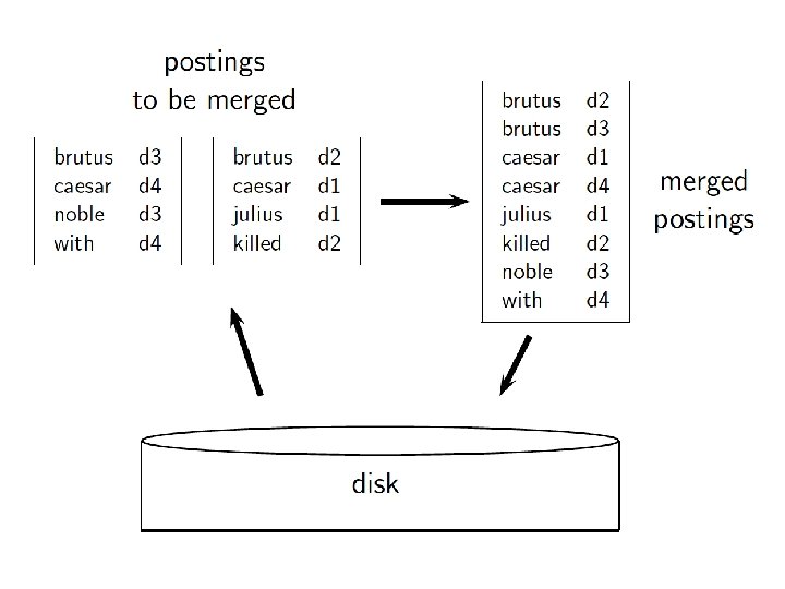
Sort based Index construction • Say we have 12 byte records - Generated as we parse docs. • Must now sort 100 M of such 12 byte records by term. • Define a Chunk to be 10 M such records - Can easily fit a couple into memory. - Will have 10 such chunks to start with. • Basic idea of algorithm: - Accumulate records for each chunk, sort, write to disk. - Then merge the chunks into one long sorted order.

Another Idea • Key idea 2: Accumulate records in postings lists as they occur. • This way we can generate a complete inverted index for each chunk. • These separate indexes can then be merged into one big index.