Index Construction sorting Paolo Ferragina Dipartimento di Informatica

Index Construction: sorting Paolo Ferragina Dipartimento di Informatica Università di Pisa Reading Chap 4

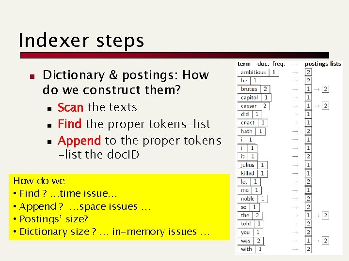
Indexer steps n Dictionary & postings: How do we construct them? n n n Scan the texts Find the proper tokens-list Append to the proper tokens -list the doc. ID How do we: • Find ? …time issue… • Append ? …space issues … • Postings’ size? • Dictionary size ? … in-memory issues …

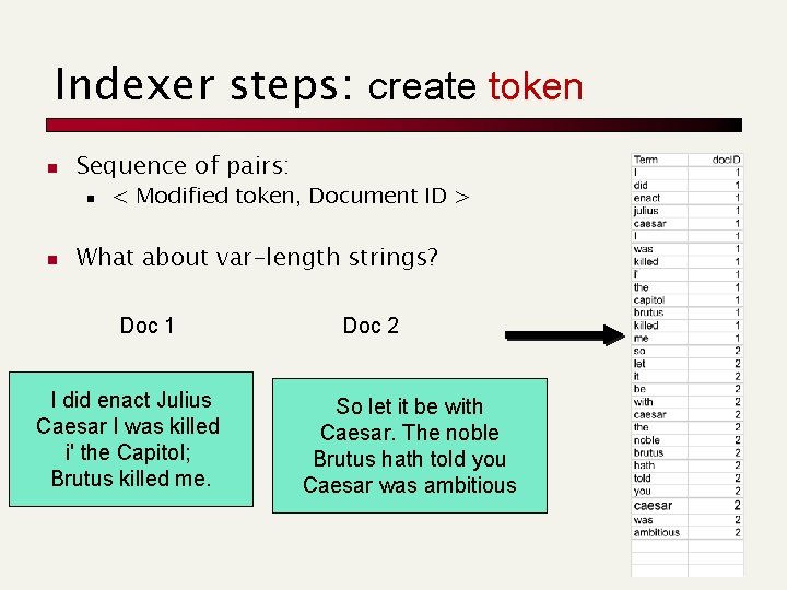
Indexer steps: create token n Sequence of pairs: n n < Modified token, Document ID > What about var-length strings? Doc 1 I did enact Julius Caesar I was killed i' the Capitol; Brutus killed me. Doc 2 So let it be with Caesar. The noble Brutus hath told you Caesar was ambitious

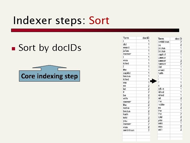
Indexer steps: Sort n Sort by doc. IDs Core indexing step

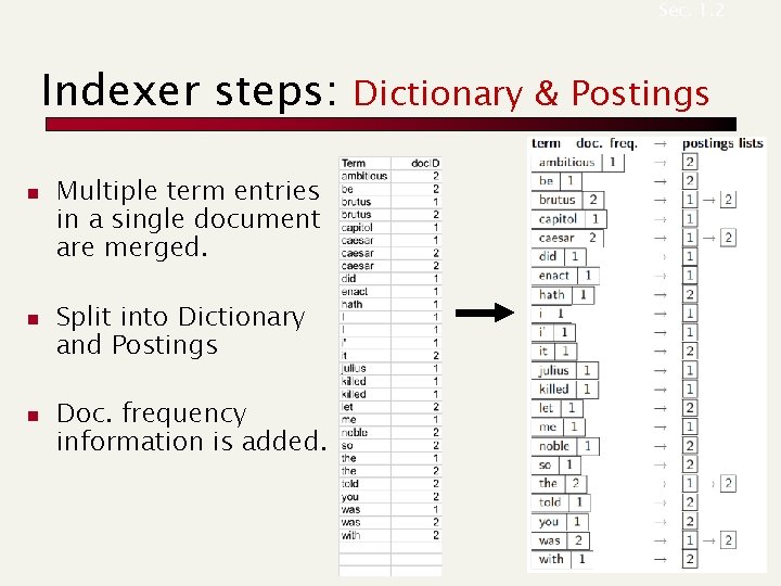
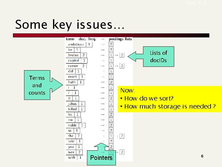
Sec. 1. 2 Indexer steps: n n n Multiple term entries in a single document are merged. Split into Dictionary and Postings Doc. frequency information is added. Dictionary & Postings

Sec. 1. 2 Some key issues… Lists of doc. IDs Terms and counts Now: • How do we sort? • How much storage is needed ? Pointers 6

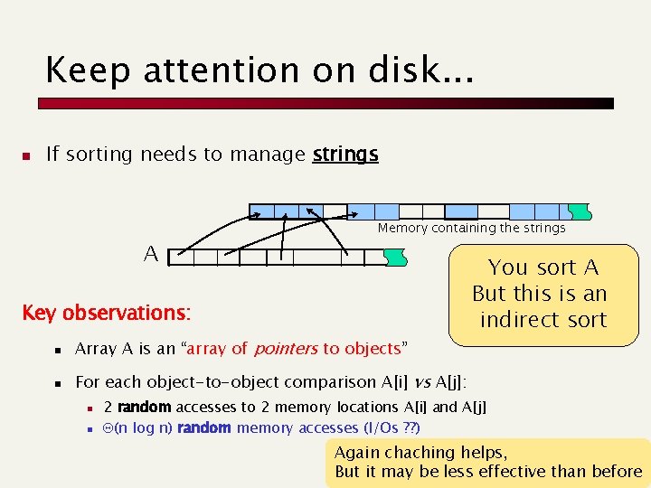
Keep attention on disk. . . n If sorting needs to manage strings A Memory containing the strings Key observations: n Array A is an “array of pointers to objects” n For each object-to-object comparison A[i] vs A[j]: n n You sort A But this is an indirect sort 2 random accesses to 2 memory locations A[i] and A[j] Q(n log n) random memory accesses (I/Os ? ? ) Again chaching helps, But it may be less effective than before

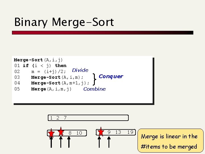
Binary Merge-Sort(A, i, j) 01 if (i < j) then 02 m = (i+j)/2; Divide Conquer 03 Merge-Sort(A, i, m); 04 Merge-Sort(A, m+1, j); 05 Merge(A, i, m, j) Combine 1 2 7 1 2 8 10 7 9 13 19 Merge is linear in the #items to be merged

Few key observations n Items = (short) strings = atomic. . . n On english wikipedia, about 109 tokens to sort n Q(n log n) memory accesses (I/Os ? ? ) n [5 ms] * n log 2 n ≈ 3 years In practice it is a “faster”, why?

Use the same algorithm for disk? n multi-way merge-sort aka BSBI: Blocked sort-based Indexing n Mapping term. ID n n n to be kept in memory for constructing the pairs Consumes memory to pairs’ creation Needs two passes, unless you use hashing and thus some probability of collision.

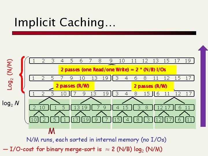
Log 2 (N/M) Implicit Caching… 1 3 4 5 6 7 8 9 10 11 12 13 15 17 19 15 17 12 17 2 passes (one Read/one Write) = 2 * (N/B) I/Os 1 2 5 7 9 10 13 19 3 4 2 passes (R/W) 1 log 2 N 2 2 2 10 10 2 5 10 7 9 1 5 13 19 5 1 13 19 6 8 11 12 2 passes (R/W) 13 19 7 9 9 7 3 4 4 15 15 4 8 15 6 11 3 8 12 17 8 3 12 17 M N/M runs, each sorted in internal memory (no I/Os) — I/O-cost for binary merge-sort is ≈ 2 (N/B) log 2 (N/M) 6 11

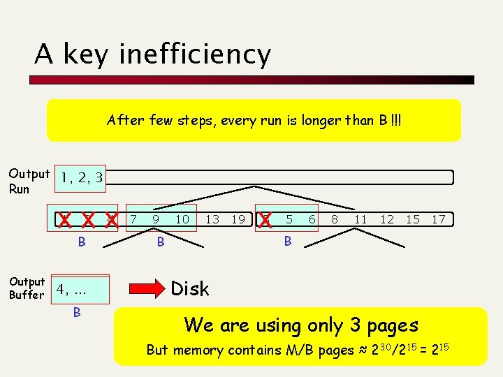
A key inefficiency After few steps, every run is longer than B !!! Output 1, 2, 3 Run 1 2 B Output Buffer 1, 4, 2, . . . 3 B 4 7 9 10 13 19 3 5 6 8 11 12 15 17 B B Disk We are using only 3 pages But memory contains M/B pages ≈ 230/215 = 215

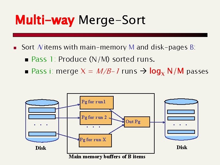
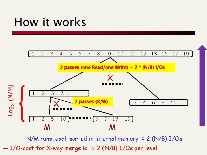
Multi-way Merge-Sort n Sort N items with main-memory M and disk-pages B: n Pass 1: Produce (N/M) sorted runs. n Pass i: merge X = M/B-1 runs log. X N/M passes Pg for run 1 . . . Pg for run 2 . . . Out Pg . . . Pg for run X Disk Main memory buffers of B items

How it works 1 2 3 4 5 6 7 8 9 10 11 12 13 15 17 19 2 passes (one Read/one Write) = 2 * (N/B) I/Os Log. X (N/M) X 1 2 5 7…. X 1 2 M 5 2 passes (R/W) 10 7 9 3 13 M 4 6 8 11…. . 19 N/M runs, each sorted in internal memory = 2 (N/B) I/Os — I/O-cost for X-way merge is ≈ 2 (N/B) I/Os per level

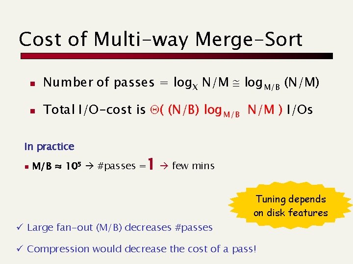
Cost of Multi-way Merge-Sort n Number of passes = log. X N/M log. M/B (N/M) n Total I/O-cost is Q( (N/B) log. M/B N/M ) I/Os In practice n M/B ≈ 105 #passes =1 few mins Tuning depends on disk features ü Large fan-out (M/B) decreases #passes ü Compression would decrease the cost of a pass!

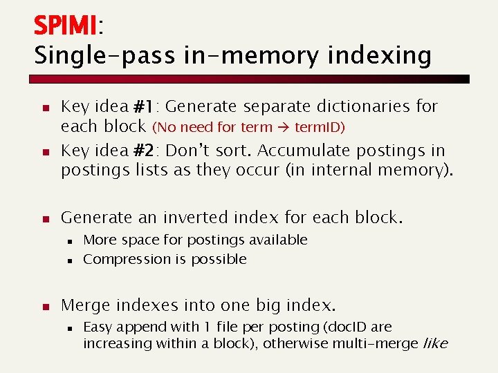
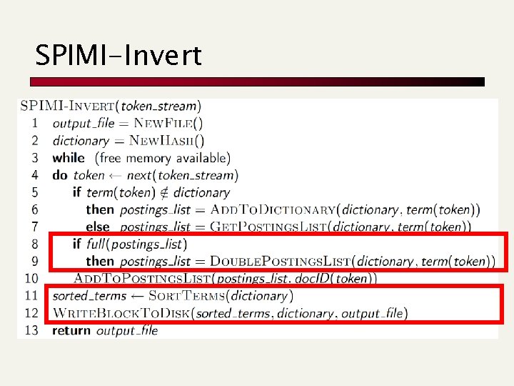
SPIMI: Single-pass in-memory indexing n n n Key idea #1: Generate separate dictionaries for each block (No need for term. ID) Key idea #2: Don’t sort. Accumulate postings in postings lists as they occur (in internal memory). Generate an inverted index for each block. n n n More space for postings available Compression is possible Merge indexes into one big index. n Easy append with 1 file per posting (doc. ID are increasing within a block), otherwise multi-merge like

SPIMI-Invert

Distributed indexing n For web-scale indexing: must use a distributed computing cluster of PCs n Individual machines are fault-prone n Can unpredictably slow down or fail n How do we exploit such a pool of machines?

Google data centers n n n Google data centers mainly contain commodity machines. Data centers are distributed around the world. Estimate: Google installs 100, 000 servers each quarter. n Based on expenditures of 200– 250 million dollars per year

Distributed indexing n n Maintain a master machine directing the indexing job – considered “safe”. Break up indexing into sets of (parallel) tasks. Master machine assigns tasks to idle machines Other machines can play many roles during the computation

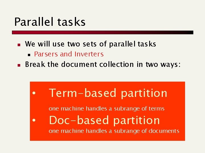
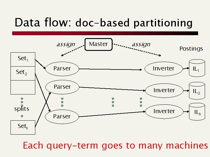
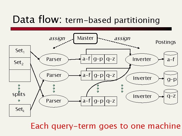
Parallel tasks n We will use two sets of parallel tasks n n Parsers and Inverters Break the document collection in two ways: • Term-based partition one machine handles a subrange of terms • Doc-based partition one machine handles a subrange of documents

Data flow: doc-based partitioning assign Master assign Postings Set 1 Set 2 Parser splits Parser Inverter IL 1 Inverter IL 2 Inverter ILk Setk Each query-term goes to many machines

Data flow: assign term-based partitioning Master assign Postings Set 1 Set 2 splits Parser a-f g-p q-z Inverter a-f Inverter g-p Inverter q-z Setk Each query-term goes to one machine

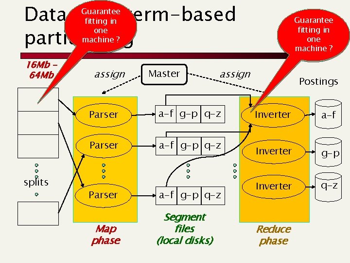
Map. Reduce n This is n n n a robust and conceptually simple framework for distributed computing … without having to write code for the distribution part. Google indexing system (ca. 2002) consists of a number of phases, each implemented in Map. Reduce.

Data flow: term-based partitioning Guarantee fitting in one machine ? 16 Mb 64 Mb splits assign Master assign Parser a-f g-p q-z Parser Map phase a-f g-p q-z Segment files (local disks) Guarantee fitting in one machine ? Postings Inverter a-f Inverter g-p Inverter q-z Reduce phase

Dynamic indexing n Up to now, we have assumed static collections. n Now more frequently occurs that: n n n Documents come in over time Documents are deleted and modified And this induces: n n Postings updates for terms already in dictionary New terms added/deleted to/from dictionary

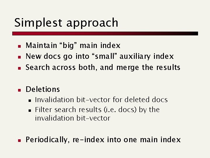
Simplest approach n Maintain “big” main index New docs go into “small” auxiliary index Search across both, and merge the results n Deletions n n n Invalidation bit-vector for deleted docs Filter search results (i. e. docs) by the invalidation bit-vector Periodically, re-index into one main index

Issues with 2 indexes n Poor performance n n n Merging of the auxiliary index into the main index is efficient if we keep a separate file for each postings list. Merge is the same as a simple append [new doc. IDs are greater]. But this needs a lot of files – inefficient for O/S. Assumption: The index is one big file. In reality: Use a scheme somewhere in between (e. g. , split very large postings lists, collect postings lists of length 1 in one file etc. )

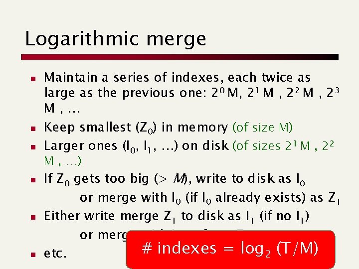
Logarithmic merge n n n Maintain a series of indexes, each twice as large as the previous one: 20 M, 21 M , 22 M , 23 M, … Keep smallest (Z 0) in memory (of size M) Larger ones (I 0, I 1, …) on disk (of sizes 21 M , 22 M , …) If Z 0 gets too big (> M), write to disk as I 0 or merge with I 0 (if I 0 already exists) as Z 1 Either write merge Z 1 to disk as I 1 (if no I 1) or merge with I 1 to form Z 2 # indexes = log 2 (T/M) etc.

Some analysis n n (T = #postings = #tokens) Auxiliary and main index: index construction time is O(T 2) as each posting is touched in each merge. Logarithmic merge: Each posting is merged O(log (T/M) ) times, so complexity is O( T log (T/M) ) Logarithmic merge is more efficient for index construction, but its query processing requires the merging of O( log (T/M) ) lists of results

Web search engines n Most search engines now support dynamic indexing n n News items, blogs, new topical web pages But (sometimes/typically) they also periodically reconstruct the index n Query processing is then switched to the new index, and the old index is then deleted

Query processing: optimizations Paolo Ferragina Dipartimento di Informatica Università di Pisa Reading 2. 3

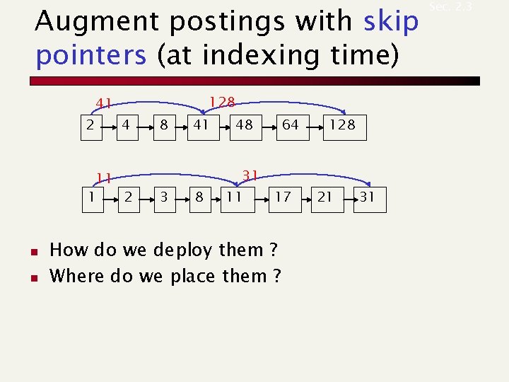
Augment postings with skip pointers (at indexing time) 2 41 128 4 11 1 2 n n 8 3 41 48 8 31 11 64 17 How do we deploy them ? Where do we place them ? 128 21 31 Sec. 2. 3

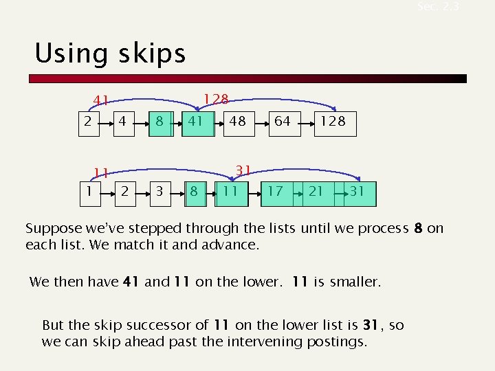
Sec. 2. 3 Using skips 2 41 128 4 11 1 2 8 3 41 48 8 31 11 64 17 128 21 31 Suppose we’ve stepped through the lists until we process 8 on each list. We match it and advance. We then have 41 and 11 on the lower. 11 is smaller. But the skip successor of 11 on the lower list is 31, so we can skip ahead past the intervening postings.

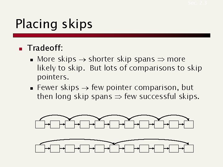
Sec. 2. 3 Placing skips n Tradeoff: n n More skips shorter skip spans more likely to skip. But lots of comparisons to skip pointers. Fewer skips few pointer comparison, but then long skip spans few successful skips.

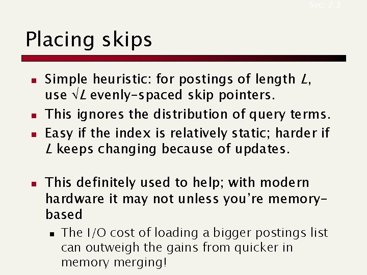
Sec. 2. 3 Placing skips n n Simple heuristic: for postings of length L, use L evenly-spaced skip pointers. This ignores the distribution of query terms. Easy if the index is relatively static; harder if L keeps changing because of updates. This definitely used to help; with modern hardware it may not unless you’re memorybased n The I/O cost of loading a bigger postings list can outweigh the gains from quicker in memory merging!

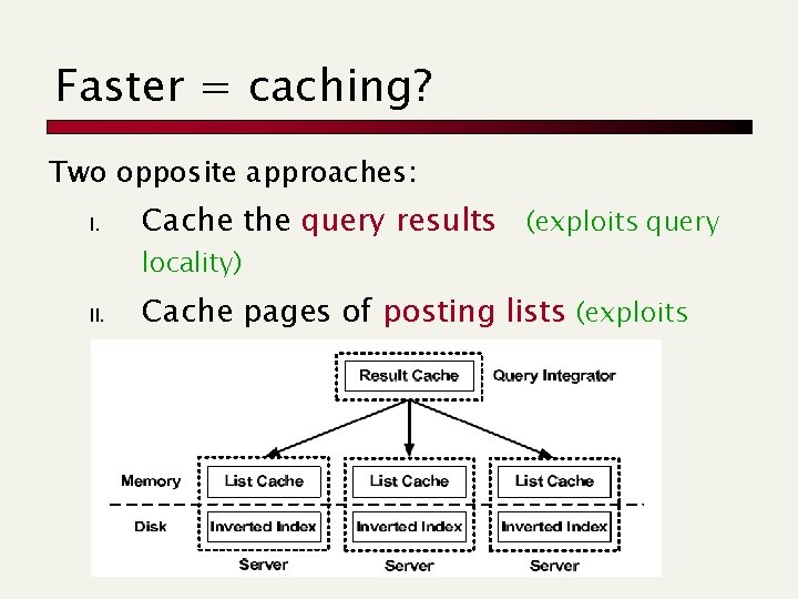
Faster = caching? Two opposite approaches: I. Cache the query results (exploits query locality) II. Cache pages of posting lists (exploits term locality)

Query processing: phrase queries and positional indexes Paolo Ferragina Dipartimento di Informatica Università di Pisa Reading 2. 4

Sec. 2. 4 Phrase queries n n Want to be able to answer queries such as “stanford university” – as a phrase Thus the sentence “I went at Stanford my university” is not a match.

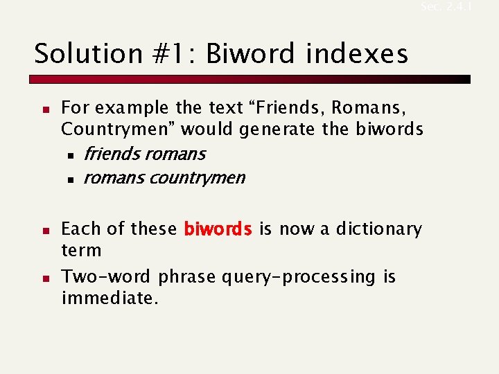
Sec. 2. 4. 1 Solution #1: Biword indexes n n n For example the text “Friends, Romans, Countrymen” would generate the biwords n friends romans n romans countrymen Each of these biwords is now a dictionary term Two-word phrase query-processing is immediate.

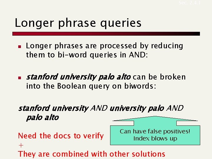
Sec. 2. 4. 1 Longer phrase queries n n Longer phrases are processed by reducing them to bi-word queries in AND: stanford university palo alto can be broken into the Boolean query on biwords: stanford university AND university palo AND palo alto Can have false positives! Index blows up Need the docs to verify + They are combined with other solutions

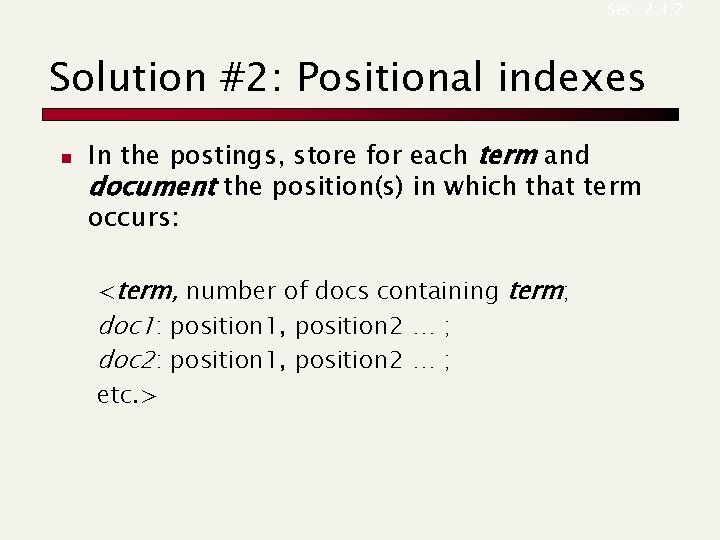
Sec. 2. 4. 2 Solution #2: Positional indexes n In the postings, store for each term and document the position(s) in which that term occurs: <term, number of docs containing term; doc 1: position 1, position 2 … ; doc 2: position 1, position 2 … ; etc. >

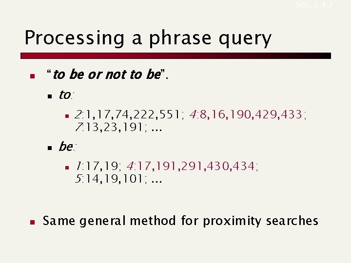
Sec. 2. 4. 2 Processing a phrase query n “to be or not to be”. n to: n n be: n n 2: 1, 17, 74, 222, 551; 4: 8, 16, 190, 429, 433; 7: 13, 23, 191; . . . 1: 17, 19; 4: 17, 191, 291, 430, 434; 5: 14, 19, 101; . . . Same general method for proximity searches

Sec. 7. 2. 2 Query term proximity n n n Free text queries: just a set of terms typed into the query box – common on the web Users prefer docs in which query terms occur within close proximity of each other Would like scoring function to take this into account – how?

Sec. 2. 4. 2 Positional index size n n n You can compress position values/offsets Nevertheless, a positional index expands postings storage by a factor 2 -4 in English Nevertheless, a positional index is now commonly used because of the power and usefulness of phrase and proximity queries … whether used explicitly or implicitly in a ranking retrieval system.

Sec. 2. 4. 3 Combination schemes n Bi. Word + Positional index is a profitable combination n For particular phrases (“Michael Jackson”, “Britney Spears”) it is inefficient to keep on merging positional postings lists better to store a bi-word n More complicated mixing strategies do exist!

Sec. 7. 2. 3 Soft-AND n E. g. query rising interest rates n Run the query as a phrase query n If <K docs contain the phrase rising interest rates, run the two phrase queries rising interest and interest rates n If we still have <K docs, run the “vector space query” rising interest rates n Rank matching docs

Query processing: other sophisticated queries Paolo Ferragina Dipartimento di Informatica Università di Pisa Reading 3. 2 and 3. 3

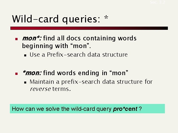
Sec. 3. 2 Wild-card queries: * n mon*: find all docs containing words beginning with “mon”. n n Use a Prefix-search data structure *mon: find words ending in “mon” n Maintain a prefix-search data structure for reverse terms. How can we solve the wild-card query pro*cent ?

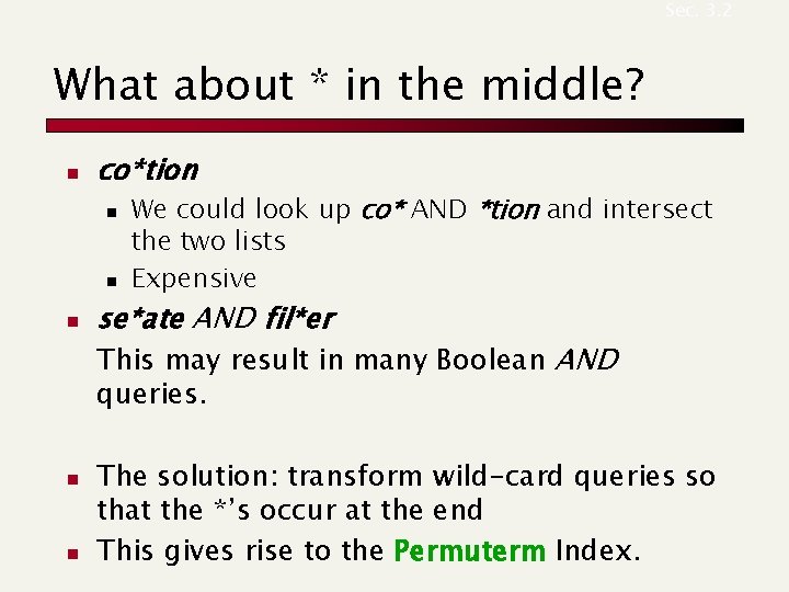
Sec. 3. 2 What about * in the middle? n co*tion n We could look up co* AND *tion and intersect the two lists Expensive se*ate AND fil*er This may result in many Boolean AND queries. n n The solution: transform wild-card queries so that the *’s occur at the end This gives rise to the Permuterm Index.

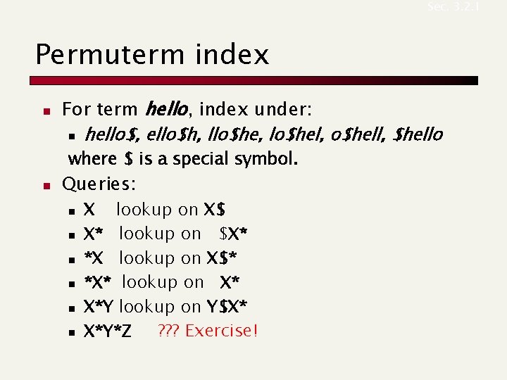
Sec. 3. 2. 1 Permuterm index n For term hello, index under: n hello$, ello$h, llo$he, lo$hel, o$hell, $hello where $ is a special symbol. n Queries: n n n X lookup on X$ X* lookup on $X* *X lookup on X$* *X* lookup on X* X*Y lookup on Y$X* X*Y*Z ? ? ? Exercise!

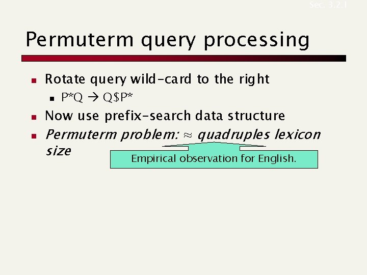
Sec. 3. 2. 1 Permuterm query processing n Rotate query wild-card to the right n n n P*Q Q$P* Now use prefix-search data structure Permuterm problem: ≈ quadruples lexicon size Empirical observation for English.

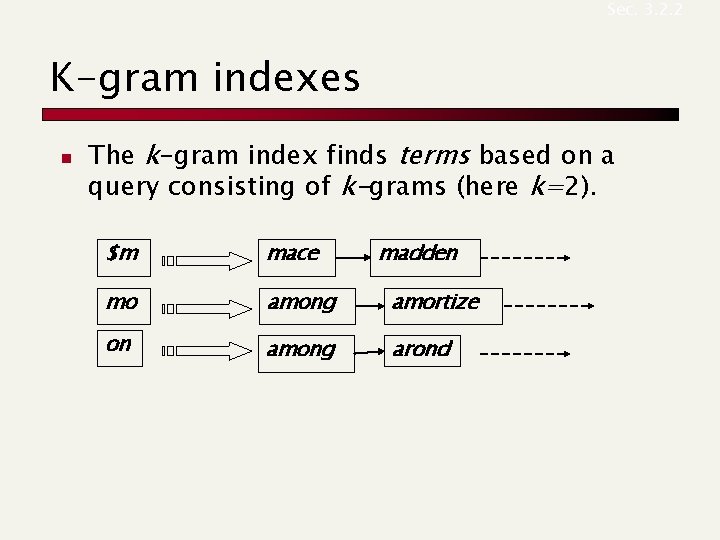
Sec. 3. 2. 2 K-gram indexes n The k-gram index finds terms based on a query consisting of k-grams (here k=2). $m mace madden mo among amortize on among arond

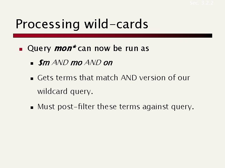
Sec. 3. 2. 2 Processing wild-cards n Query mon* can now be run as n $m AND mo AND on n Gets terms that match AND version of our wildcard query. n Must post-filter these terms against query.

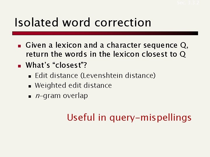
Sec. 3. 3. 2 Isolated word correction n n Given a lexicon and a character sequence Q, return the words in the lexicon closest to Q What’s “closest”? n n n Edit distance (Levenshtein distance) Weighted edit distance n-gram overlap Useful in query-mispellings

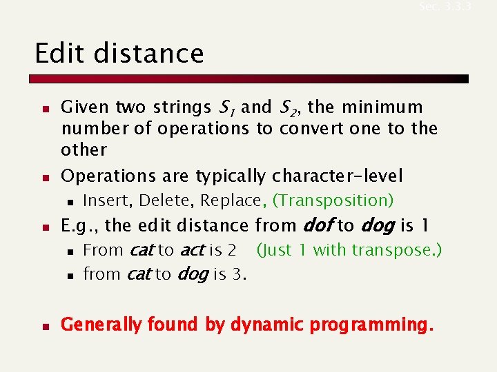
Sec. 3. 3. 3 Edit distance n n Given two strings S 1 and S 2, the minimum number of operations to convert one to the other Operations are typically character-level n n n Insert, Delete, Replace, (Transposition) E. g. , the edit distance from dof to dog is 1 n From cat to act is 2 (Just 1 with transpose. ) n from cat to dog is 3. Generally found by dynamic programming.

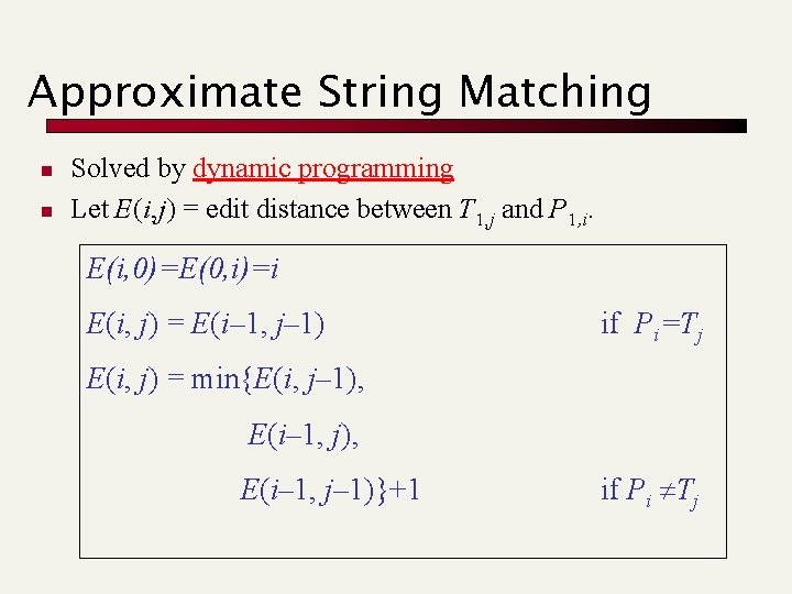
Approximate String Matching n n Solved by dynamic programming Let E(i, j) = edit distance between T 1, j and P 1, i. E(i, 0)=E(0, i)=i E(i, j) = E(i– 1, j– 1) if Pi=Tj E(i, j) = min{E(i, j– 1), E(i– 1, j– 1)}+1 if Pi Tj

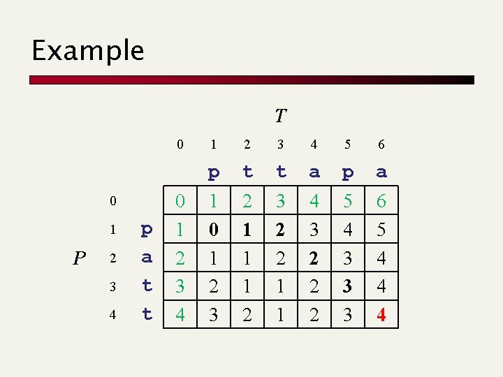
Example T 0 0 1 P 2 3 4 p a t t 0 1 2 3 4 5 6 p t t a p a 1 0 1 2 3 2 1 1 1 2 3 2 2 1 1 4 3 2 2 2 5 4 3 3 3 6 5 4 4 4

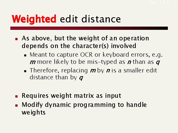
Sec. 3. 3. 3 Weighted edit distance n As above, but the weight of an operation depends on the character(s) involved n n Meant to capture OCR or keyboard errors, e. g. m more likely to be mis-typed as n than as q Therefore, replacing m by n is a smaller edit distance than by q Requires weight matrix as input Modify dynamic programming to handle weights

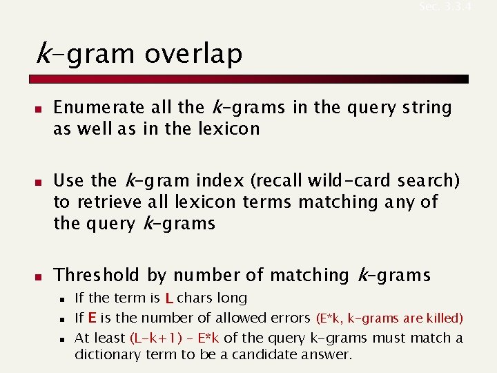
Sec. 3. 3. 4 k-gram overlap n n n Enumerate all the k-grams in the query string as well as in the lexicon Use the k-gram index (recall wild-card search) to retrieve all lexicon terms matching any of the query k-grams Threshold by number of matching k-grams n n n If the term is L chars long If E is the number of allowed errors (E*k, k-grams are killed) At least (L-k+1) – E*k of the query k-grams must match a dictionary term to be a candidate answer.

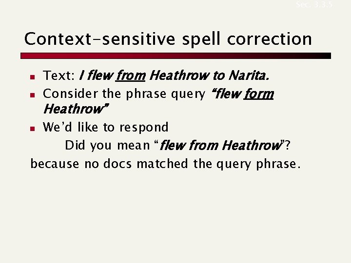
Sec. 3. 3. 5 Context-sensitive spell correction n n Text: I flew from Heathrow to Narita. Consider the phrase query “flew form Heathrow” We’d like to respond Did you mean “flew from Heathrow”? because no docs matched the query phrase. n