INDEPENDENT SAMPLES TTESTS TwoSample tTests 1 Distinguish between

INDEPENDENT SAMPLES TTESTS

Two-Sample t-Tests 1. Distinguish between the statistical question underlying CIs, 1 -sample hypothesis tests and 2 sample hypothesis tests. 2. Describe the procedures for conducting independent 2 -sample hypothesis tests when σ is known. • calculation of standard error • calculation/interpretation of CI 3. Describe the procedures for conducting independent 2 -sample hypothesis tests when σ is unknown. • calculation of pooled estimate of variance • calculation of standard error • calculation/interpretation of CI 4. Compare the results of tests conducted using the small and large-sample methods.

Important Questions Confidence Interval: ■ What is the range within which we can be (1 - )% sure that falls? 1 -Sample Hypothesis Test: ■ What is the likelihood that the sample we have collected was drawn from a population with = ___? 2 -Sample Hypothesis Test: ■ What is the likelihood that two samples we have collected were drawn from populations with the same value for ?

2 Types of 2 -Sample Tests Paired test – two conditions are comprised of the same elements; same observation is measured under different testing conditions. – EX: Independent test – two conditions are comprised of different elements/observations; often called unpaired – EX:

Comparing one- & two-sample tests 1 Sample Tests: – Ho: μ = some value – Ha: μ ≠ some value – Observed value of test stat = 2 Sample Tests: – Ho: μ 1 = μ 2 – Ha: μ 1 ≠ μ 2 – Observed value of test stat =

Sampling Distribution of Differences Between Means The distribution of the differences between means over repeated sampling from the same population Where does the difference we observe between our samples fall if we assume the null is true? Ha: 1 - 2 0 0

2 -sample Hypothesis Test Step 1: Decide whether to conduct a one or a two-tailed test. § We’ll start with two-tailed tests. Steps 2 and 3: Set up your null and alternative hypotheses Ho: 1 - 2 = 0 or 1 = 2 Ha: 1 - 2 0 or 1 2 Step 4: Choose alpha

2 -sample Hypothesis Test Step 5: Set up a Rejection Region by determining zcrit or tcrit Step 6: Calculate zobs or tobs Step 7: Make a decision regarding the null. § Crit Value: Does the observed value of your test statistic fall in the rejection region? § P-value: Is our observed probability less than what alpha is set to? Step 8: Interpret what your decision regarding the null means in terms of your original research question.

Do incentives increase innovation? The boss of a tech development firm wants to boost creativity among her employees. To examine if incentives will help, she randomly assigns employees (n = 36) to an incentive condition or to a control condition (n = 36). Those in the incentive condition are told that they will be rewarded with a bonus for each new proposal that demonstrates high innovation. The control condition is told nothing. The boss then measures the number of proposals made by each employee that meet her criteria of innovation. Does the boss have sufficient evidence to conclude that incentives increase innovation? α =. 05. Control Mc = 3. 5 proposals σc = 1. 4 Incentives Min = 2. 1 proposals σin = 0. 8

Do incentives increase innovation? Control Mc = 3. 5 proposals σc = 1. 4 Incentives Min = 2. 1 proposals σin = 0. 8 Step 1: Let’s conduct a two-tailed test. Steps 2 and 3: Set up your null and alternative hypotheses Ho: c - in = 0 or c = in Ha: c - in 0 or c in Step 4: α =. 05. Step 5: zcrit = ± 1. 96

Do incentives increase innovation? ■

Do incentives increase innovation? Control Mc = 3. 5 proposals σin = 1. 4 n = 36 Step 6: Calculate zobs SE: Incentives Mc = 2. 1 proposals σin = 0. 8 n = 36

Null hypothesis sampling distribution of differences between means μ 1 -μ 2=0 Zobs=5. 19 -1. 96 +1. 96

Do incentives increase innovation? Control Mc = 3. 5 proposals σin = 1. 4 Incentives Mc = 2. 1 proposals σin = 0. 8 Zcrit = ± 1. 96 Zobs = 5. 19 Decision: we will reject the null because Zobs falls in the rejection region z = 5. 19, p <. 05 Interpretation: Incentives significantly decreased the average number of innovative proposals made by employees

What does statistical significance We expect some amount of error or variability from sample to mean? sample. A hypothesis test evaluates whethere is more variability or error than we would expect. § We reject the null if the observed error is significantly larger than we’d expect by chance. 1 -sample test: § If the difference between M and 0 is significantly larger than we would expect by chance, we conclude that there is a significant difference between and 0. 2 -sample test: § If the difference between M 1 and M 2 is significantly larger than we would expect by chance, we conclude that there is a significant difference between 1 and 2.

Two-Sample Test: Anthropology An anthropologist wants to collect data to determine whether the two different cultural groups that occupy an isolated Pacific Island grow to be different heights. The results of his samples of the heights of adult females are as follows. Group A n = 120 M = 62. 7 σ = 2. 5 Group B n = 120 M = 61. 8 σ = 2. 62 Do these samples constitute enough evidence to reject the null hypothesis that the heights of the two groups are the same? Set alpha to. 05.

Two-Sample Test: Anthropology Group A n = 120 M = 62. 7 σ = 2. 5 Group B n = 120 M = 61. 8 σ = 2. 62 Step 1: Run a two-tailed test. Step 2: Ho: a = b Step 3: Ha: a b Steps 4 and 5: α =. 05; zcrit = ± 1. 96

Two-Sample Test: Anthropology Group A n = 120 M = 62. 7 σ = 2. 5 Group B n = 120 M = 61. 8 σ = 2. 62 Step 6: = 2. 73 Step 7: Decision regarding the null? (zcrit = ± 1. 96) Step 8: Interpretation

Observed p-value method zobs = 2. 73 Proportion in tail =. 0032 P-value: . 0032 x 2 =. 0064 . 0032 -2. 73 . 0032 +2. 73

Observed p-value method zobs = 2. 73 Proportion in tail =. 0032 P-value: . 0032 x 2 =. 0064 Decision: . 0064 is less than alpha (. 05), reject the null § Z = 2. 73, p =. 0064 § “the probability of getting a mean difference at least as extreme as the one we got if the null is true is. 0064”

When to do a t-test We should use t instead of z if the σ is unknown We also have to use t instead of z if we have small sample sizes § (because the CLT can no longer be applied) When using t: § df = (n-1)+(n-1) =n+n-2 § If group n’s are equal SE is calculated the same:

Independent Sample t-test steps Step 1: One- vs. Two-tailed test Step 2: Specify the NULL hypothesis (HO) § 1 = 2 OR 1 - 2 = 0 Step 3: Specify the ALTERNATIVE hypothesis (Ha) § 1 2 OR 1 - 2 0 Step 4: Designate the rejection region by selecting . Step 5: Determine the critical value of your test statistic § df = (n 1+n 2) – 2

Independent Sample t-test steps Step 6: Calculate the SE and t observed. Step 7: Compare observed value with critical value: § If test statistic falls in RR, we reject the null. § Otherwise, we fail to reject the null. Step 8: Interpret your decision regarding the null in terms of your original research question.

Bruno’s vs. Sibies It’s late at night and you have been partying working HARD! It’s time for a little snack, but you have miles to go before you sleep so you need your pizza delivered FAST. Below are delivery times for recent orders from two local establishments. Do these data provide enough evidence to conclude that one delivers pizza more quickly ( =. 05)? Bruno’s 33 35 32 31 M = 32 29 s = 2. 24 35 38 M = 36 Sibies 37 37 33 s = 2. 00

Bruno’s 33 35 32 31 M = 32 29 s = 2. 24 35 38 Sibies 37 37 M = 36 Step 1: run a two-tailed test. Step 2: Ho: B= S Step 3: Ha: B S Step 4: α =. 05 Step 5: df = n+n-2= 5+5 -2= 8; tcrit = ± 2. 306 33 s = 2. 00

Bruno’s 33 35 32 31 M = 32 29 s = 2. 24 Step 6 a: calculate SE 35 38 M = 36 Sibies 37 37 33 s = 2. 00

Bruno’s 33 35 32 31 M = 32 29 s = 2. 24 Step 6 a: calculate SE obs 35 38 M = 36 Sibies 37 37 33 s = 2. 00 Step 6 b: calculate t-

Bruno’s M = 32 s = 2. 24 Sibies M = 36 s = 2. 00 Step 7: Decision regarding the null: reject Step 8: Interpretation: Mean delivery time for Bruno’s (M = 32, SD = 2. 24) was significantly faster than mean delivery time for Sibies (M = 36, SD = 2. 00), t(8) = -2. 98, p <. 05

Important Note About SE Calculating SE with this formula only is appropriate if our groups have equal n’s If sample sizes are unequal we must calculate a pooled variance (Sp 2)
 We have to calculate a weighted average: 1.")
Calculating a Pooled Variance (Sp 2) We have to calculate a weighted average: 1. 2. Standard error: Remember SS= sums of squared deviations: (equal to the numerator of the formula for variance)

Bruno’s 33 35 32 31 M = 32 29 s = 2. 24 Step 6: Calculate S 2 p 35 38 M = 36 Sibies 37 37 33 s = 2. 00
 = 160 29 s =")
Bruno’s 33 35 32 31 M = 32 (x) = 160 29 s = 2. 24 (x 2) = 5140 35 38 Sibies 37 37 M = 36 (x) = 180 33 s = 2. 00 (x 2) = 6496 Step 6: Calculate S 2 p (x 1) = 160 (x 12) = 5140 (x 2) = 180 (x 22) = 6496
 = 160 29 s =")
Bruno’s 33 35 32 31 M = 32 (x) = 160 29 s = 2. 24 (x 2) = 5140 35 38 Sibies 37 37 M = 36 (x) = 180 33 s = 2. 00 (x 2) = 6496 S 2 p = 4. 5 Step 6 a: Calculate SE (same for both methods)
 = 160 29 s =")
Bruno’s 33 35 32 31 M = 32 (x) = 160 29 s = 2. 24 (x 2) = 5140 35 38 M = 36 (x) = 180 Step 7: Calculate tobs Step 8: Decision Regarding the null Step 9: Interpretation Sibies 37 37 33 s = 2. 00 (x 2) = 6496

Advil I am of the opinion that Advil doesn't really work. I feel like, eventually, my headache goes away whether or not I take Advil. So, for the past few months, I have been measuring how long it takes for my headache to go away when I use Advil compared to when I do not. On average, the 15 headaches for which I used Advil went away in 19 minutes (SD = 6), and the 11 headaches for which I did not use Advil went away in 23 minutes (SD = 8). Do these data constitute enough evidence to conclude that Advil is effective in treating headaches ( =. 01)?

Hypnosis and eye witness testimony People who witness a crime may recall the details of the crime differently when under hypnosis. Participants are asked to watch a video of a robbery and half are randomly assigned to a hypnosis condition. These subjects are hypnotized and then asked 30 questions about the robbery. The other participants answer the same questions without being hypnotized. α =. 05 Hypnosis No Hypnosis Mean correct responses 23 20 Number of participants 17 15 Estimated Variance 9. 0 7. 5 1. ) Conduct a two samples t-test 2. ) Calculate and interpret the 95% CI 3. ) Calculate and interpret Cohen’s D

Hypnosis No Hypnosis Mean number of questions correct 23 20 Number of participants 17 15 Estimated Variance 9. 0 7. 5 Step 1: Run a two-tailed test Step 2: µh = µnh Step 3: µh µnh Steps 4 and 5: α =. 05; df = 30; tcrit = ± 2. 042

Hypnosis No Hypnosis Mean number of questions correct 23 20 Number of participants 17 15 Estimated Variance 9. 0 7. 5 Step 6:

Hypnosis and eye witness testimony Step 7: Decision regarding the null: reject the null, tobs is in the rejection region Step 8: interpretation: Subjects answered significantly more questions correctly when hypnotized (M = 23) than when not (M = 20), t (30) = 2. 93, p <. 05
 t /2 (σM")
Hypnosis and eye witness testimony 95 % Confidence interval: (MHyp-MNo. Hyp) t /2 (σM 1 -M 2) (23 -20) 2. 042 (1. 023) 95% CI [0. 911, 5. 089] We are 95% confident that the population mean difference in correct answers between people under hypnosis and those not under hypnosis is between. 91 and 5. 09

Hypnosis and eye witness testimony Effect size: Cohen’s d = This is a large effect.

Reporting results of an independent ttest Individuals under hypnosis answered significantly more questions correctly (M = 23. 00, SD = 3. 00) than those not under hypnosis (M = 20. 00, SD = 2. 74), t (30) = 2. 93, p <. 05. The 95% confidence interval for the difference is 0. 91 to 5. 09. The Cohen’s D effect size is 1. 04, suggesting a large effect. Questions correct as a function of hypnosis questions correct 30 25 20 15 10 5 0 No Hypnosis

Reporting results of an independent ttest Individuals under hypnosis answered significantly more questions correctly (M = 23. 00, SD = 3. 00) than those not under hypnosis (M = 20. 00, SD = 2. 74), t (30) = 2. 93, p < . 05. The 95% confidence interval for the difference is 0. 91 to 5. 09. The Cohen’s D effect size is 1. 04, suggesting a large effect.
")
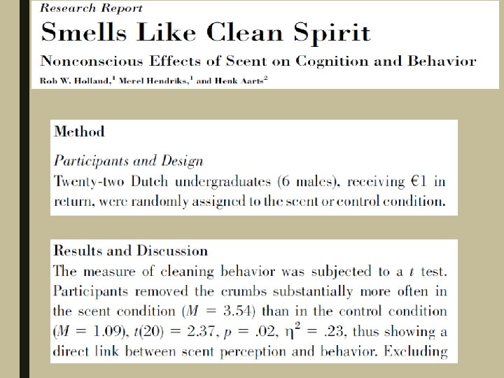
Eskine Results (you can understand them now!!!!)

Participants were randomly assigned to sit in a room with a citrus cleaner scent (clean scent) or in a room with no scent (control). Participants were then provided with a biscuit to eat. Number of times the participant removed crumbs from table was coded to measure cleaning behavior, alpha was set to. 05.

Results: Clean Scent: M = 3. 54 times Control: M = 1. 09 times t (20) = 2. 37, p =. 02 Answer the following: § What were the IV and DV? § Provide an interpretation of the results § Assuming equal sample sizes, how many subjects were in each group? (OK if you get stuck on this one)

Participants were children with and without a diagnosis of ADHD. Children and their teacher were both asked to rate the child’s social acceptance on a 1 to 4 scale, higher suggests more accepted by peers.
.")
Child’s perception of their social acceptance: ADHD: M = 2. 75 (SD =. 67). 77) Control: M = 2. 88 (SD = t(76) =. 61, p >. 05, d =. 18 Results for teacher’s rating of the child’s social acceptance: ADHD: M = 2. 12 (SD =. 67). 35) Control: M =3. 75 (SD = t(76) = 12. 01, p <. 05, d = 2. 92 Answer the following: § What was the IV and what were the two DVs?

Assumptions of independent t-tests 1. The observations in each sample must be independent 2. The two populations from which the samples are drawn must be normal § can overcome by using a large sample 3. HOMOGENEITY OF VARIANCE: The two populations from which the samples are drawn must have equal variances

Why is homogeneity of variance essential? ■ We calculate a pooled variance as the average of the two sample variances ■ This only makes sense to do this if they are estimating the same thing (the same population variance) ■ Otherwise the average is meaningless – Average of 2 IQ scores makes sense – Average of an IQ score and how fast someone can sprint 100 meters makes no sense, it’s meaningless

What if we violate this assumption? If violated, we may negate any meaningful interpretation of results § BUT Bigger issue when we have two very different sample sizes We only need to really worry if one variance is 3 -4 times larger than the other variance

Using RC Research question: Do people who identify as male vs. female differ in the number of veggies they eat per day? Alpha =. 05

RC output – Veggies x Gender Two Sample t-test data: Veggies by Gender t = 1. 733, df = 28, p-value = 0. 0941 alternative hypothesis: true difference in means is not equal to 0 95 percent confidence interval: -0. 185512 2. 223790 sample estimates: mean in group Female mean in group Male 2. 473684 1. 454545 mean sd se(mean) data: n Female 2. 473684 1. 678902 0. 3851666 19 Male 1. 454545 1. 293340 0. 3899566 11

RC output – Veggies x Gender Two Sample t-test data: Veggies by Gender t = 1. 733, df = 28, p-value = 0. 0941 alternative hypothesis: true difference in means is not equal to 0 95 percent confidence interval: -0. 185512 2. 223790 sample estimates: mean in group Female mean in group Male 2. 473684 1. 454545 mean sd se(mean) data: n Female 2. 473684 1. 678902 0. 3851666 19 Male 1. 454545 1. 293340 0. 3899566 11

RC output – Pizza Delivery Two Sample t-test data: Delivery by Pizza. Joint t = -2. 9814, df = 8, p-value = 0. 01756 alternative hypothesis: true difference in means is not equal to 0 95 percent confidence interval: -7. 0938292 -0. 9061708 sample estimates: mean in group Bruno's mean in group Sibies 32 36 mean sd se(mean) data: n Bruno's 32 2. 236068 1. 0000000 5 Sibies 36 2. 000000 0. 8944272 5

RC output – Pizza Delivery Two Sample t-test data: Delivery by Pizza. Joint t = -2. 9814, df = 8, p-value = 0. 01756 alternative hypothesis: true difference in means is not equal to 0 95 percent confidence interval: -7. 0938292 -0. 9061708 sample estimates: mean in group Bruno's mean in group Sibies 32 36 mean sd se(mean) data: n Bruno's 32 2. 236068 1. 0000000 5 Sibies 36 2. 000000 0. 8944272 5

RC output – Advil Two Sample t-test data: Relief by Prescription t = -1. 4595, df = 24, p-value = 0. 1574 alternative hypothesis: true difference in means is not equal to 0 95 percent confidence interval: -9. 656404 1. 656404 sample estimates: mean in group Advil mean in group Get. Tough 19 23 mean sd se(mean) data: n Advil 19 6 1. 549193 15 Get. Tough 23 8 2. 412091 11

RC output – Advil Two Sample t-test data: Relief by Prescription t = -1. 4595, df = 24, p-value = 0. 1574 alternative hypothesis: true difference in means is not equal to 0 95 percent confidence interval: -9. 656404 1. 656404 sample estimates: mean in group Advil mean in group Get. Tough 19 23 mean sd se(mean) data: n Advil 19 6 1. 549193 15 Get. Tough 23 8 2. 412091 11

Using SPSS Research question: Do people who identify as male vs. female differ in the number of veggies they eat per day? Alpha =. 05

SPSS output– Veggies x Gender

Using SPSS Research question: Let’s re-analyze the pizza delivery data using SPSS

SPSS output – Pizza Delivery

Factors influencing Independent Samples tests Small sample size: § Results in larger SE § Larger expected differences from sample to sample (more error) § A larger mean difference needed to detect an effect (larger t-crit value)

Factors influencing Independent Samples tests Large variance: § Results in larger SE § Larger expected differences from sample to sample (more error) § Greater difficulty detecting a systematic difference in the population
- Slides: 66