Independent Samples t test Power and Sample size

Independent Samples t test Power and Sample size 11/20/14 At the end of today’s class you can finish HW #4

Today • Quiz 6 • Assumptions of Independent samples t test. – HOV • Informal test divide larger variance by smaller if greater than 2 HOV is a problem. • Formal test is Levene’s test. Null is the variances are equal. We do not want to reject – Normality – Random assignment for causal claim – Independence • Power Analysis

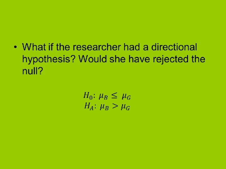
• A stronger design for last week’s weight loss program is to perform a true experiment. – Randomly assigned 20 dudes to either control or new program. – After six weeks measure their weight. – Why is the design better? • • What could be done to improve it even more? Perform non-directional Independent samples t test by hand. – See values on next slide. – Follow hypothesis testing steps in handout from last week. – Calculate Cohen’s d • At what percentile of the control is the average person in the new program? – Verify with SPSS – Construct a 95% CI around the difference in means. • See upcoming slide on Cis. Control Program 130 127 124 126 135 129 127 123 127 124 128 129 136 132 130 125 131 135 128 126

Remember you need to pool the variance, not the SD. Does it look like we have Homogeneity of Variance (HOV)? Remember you have to square the SDs to check this assumption.

Verify results with SPSS • Create one column labeled condition. – Enter 10 ones and 10 twos. • This is your independent variable. It is categorical. • If you go into variable view you can label it assigned program or something similar and assign the values with 1 = control and 2 = treatment. – In the next column enter the 10 weight values for the control and the 10 weight values for the treatment. • Then click analyze->compare means-> Independent sample t test – Place weight (your DV) in the test variable(s) box. – Place condition in the grouping variable box and click define groups. For group 1 enter 1 and group 2 enter 2. These values can be any value that you use to define the conditions. • You could have used 0 for control and 1 for treatment, or 999 for control and 2 for treatment. i. e. , it’s a nominal (categorical) variable and the number does not imply rank or degree. – Click continue then OK. • Compare results to your hand calculation. – This is what your homework requires. There should be one to one correspondence. If there is not, you made an error and might consider fixing it.

Confidence intervals • How was the 95% confidence interval calculated for the independent samples t test? – Make sure you know how to calculate for the test. – Make sure you know what value will be in or not in the interval. • If you reject the null with α =. 05 (zero will not be in 95% CI. • If you fail to reject the null with α =. 05 (zero will be in 95% CI).

How to calculate confidence intervals. From example Notice what value is contained in the 95% CI. What if I wanted a 99% CI? What α does that map on to?

One more example • A researcher is interested on whether 8 th grade boys differ from girls in attitude towards science. – She collects the following data. • Boys n = 24, mean = 62. 5, sd = 10. 2 • Girls n = 24, mean = 57. 5, sd = 9. 7 – Do we have homogeneity of variance? » SPSS had Levene’s test. The null for this test is the variances are equal the alternative is they are not equal. We don’t want to reject the null. If we do, we have to interpret the lower row of SPSS output that reads “equal variance not assumed. ” • Perform a non-directional independent samples t test with α =. 05. – Calculate Cohen’s d. • Whether significant or not. – We’re going to use it later.

Which test? • Each of the following studies requires a t test for one or more population means. Specify whether the appropriate t test is for one sample or two independent samples. – College students are randomly assigned to undergo either behavioral therapy or Gestalt therapy. After 20 therapeutic sessions, each student earns a score on a mental health questionnaire. – One hundred college freshmen are randomly assigned to sophomore roommates having either similar or dissimilar vocational goals. At the end of their freshman year, the GPAs of these 100 freshmen are to be analyzed on the basis of the previous distinction. – According to the U. S. Department of Health and Human Services, the average 16 -year-old male can do 23 push-ups. A physical education instructor finds that in his school district, 30 randomly selected 16 -yearold males can do an average of 28 push-ups. – A class of children are assessed on ability to infer the meanings of unknown words. This is followed by systematic reading instruction that emphasizes determining word meaning from context. After instruction the children are again measured on their ability to infer word meaning.

More on Statistical Significance Testing

The Problems with SST • We misunderstand what it does tell us. • It does not tell us what we want to know. • We often overemphasize SST.

Four Important Questions 1. Is there a real relationship in the population? Statistical Significance 2. How large is the relationship? Effect Size or Magnitude 3. Is it a relationship that has important, powerful, useful, meaningful implications? Practical Significance 4. Why is the relationship there? ? ? ?

SST is all about. . . • Sampling Error – The difference between what I see in my sample and what exists in the target population. – Simply because I sampled, I could be wrong.

How it works: 1. Assume sampling error occurred; there is no difference in the population. 2. Build a statistical scenario based on this null hypothesis 3. How likely is it I got the sample value I got when the null hypothesis is true? (This is the p-value. )

How it works (cont’d): • How unlikely does my result have to be to rule out sampling error? alpha ( ). • If p < , then our result is statistically rare, is unlikely to occur when there isn’t a relationship in the population.

What it does tell us • Whether sampling error is a competing hypothesis for our finding.

What it does not tell us • • • Whether the null hypothesis is true. Whether our results will replicate. Whether our research hypothesis is true. How big the effect or relationship is. How important the results are. Why there is a relationship.

Type I and II errors Power and Sample Size

Type 1 Error & Type 2 Error Scientist’s Decision Reject null hypothesis Fail to reject null hypothesis Null hypothesis is true Null hypothesis is false Type 1 Error probability = Correct Decision Probability = 1 - Correct decision probability = 1 - Type 2 Error probability = = Cases in which you reject null hypothesis when it is really true Type 2 Error = Cases in which you fail to reject null hypothesis when it is false

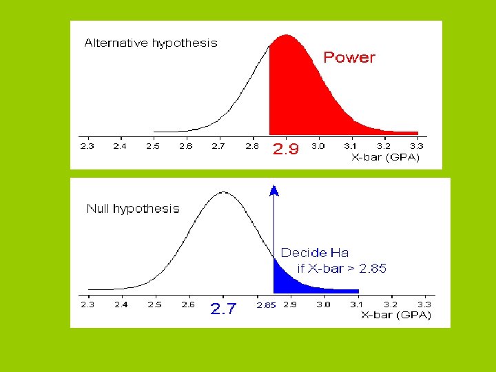
Power and sample size estimation • Power is the probability of correctly rejecting a null hypothesis (1 – β). – In social sciences we typically use. 80. – In health sciences we typically use. 95. • What determines the power of a study – – – Effect size Sample size Variance α One vs. two tailed tests

If you want to know • Sample Size – Need to know • α • β • Δ – To get Δ or d you will need variance estimates. – Where might you get them? • Power – Need to know • α • n per condition or with one-sample t test N. • Δ – To get Δ or d you will need variance estimates. – Where might you get them?

Calculating Power • Let’s say we did a study with N = 30 with the same number in each group. – We failed to reject the null. • The study may have been underpowered – How much power did the study have if d =. 30? • Go to http: //www. stat. uiowa. edu/~rlenth/Power/ • Select “two sample t test (pooled or Satterthwaite” – See tutorial on Web. Ct for more details when doing homework.

Study power

Calculating sample size • Say we want to perform a test with – power (1 -β) =. 80 – Two tailed alpha =. 05 – d =. 30 • How many participants would we need?

Solving for n: 1 -β =. 80 two-tailed

Solving for n: 1 -β =. 80 one tailed

Solving for n: 1 -β =. 95 two-tailed

Solving for n: 1 -β =. 95 one-tailed

Power and sample size for onesample t test A recent study found people to have a mean weight of 127 pounds. You suspect that people from your clinic weigh more on average. Perform a one-sample t test.

Cohen’s d for one-sample t test or paired-samples t test.

How much power did the study have?

What if we used a two-tailed test?

What if the effect size was smaller?

Calculating Power • Remember the gender difference in science perception study? • We failed to reject the null (p >. 05) – The study may have been underpowered • Calculate how much power the study had with the Cohen’s d we observed. • Calculate how many participants would be needed to have power of. 80, . 95 for both one and two tailed tests. • Tutorial on Black. Board – If you need extra help with SPSS and Piface on your homework.

Next Class 12/4 • • • Homework #4 due 12/5. Testing Pearson’s r Categorical data Course wrap-up Practice exam.